No battle plan survives contact with the enemy.
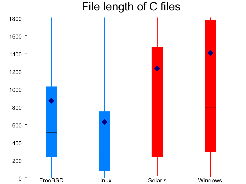
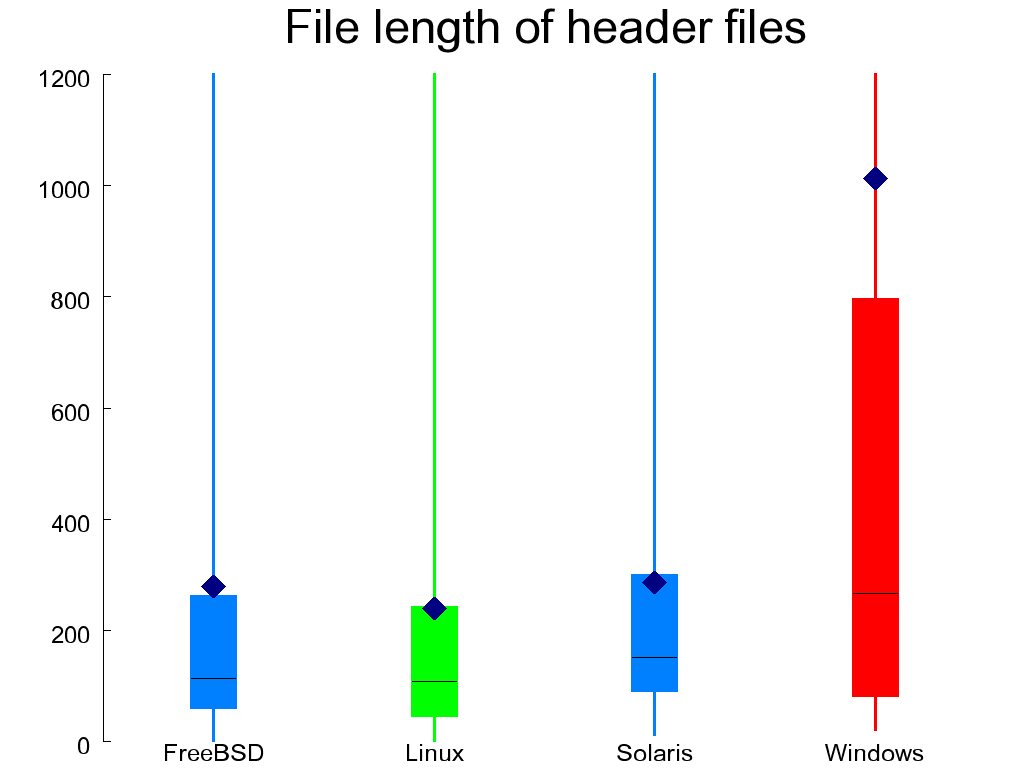
The key properties of the systems I examine appear in Table 1.1, “Key metrics of the four systems”. The quality metrics I collected can be roughly categorized into the areas of file organization, code structure, code style, preprocessing, and data organization. When it is easy to represent a metric with a single number, I list its values for each of the four systems in a table and on the left I indicate whether ideally that number should be high (↑), low (↓), or near a particular value (e.g. ≅ 1). In other cases we must look at the distribution of the various values, and for this I use so-called candlestick figures, like Figure 1.3, “File length in lines of C files (left) and headers (right)”. Each element in such a figure depicts five values:
the minimum, at the bottom of the line,
the lower (25%) quartile, at the bottom of the box,
the median (the numeric value separating the higher half of the values from the lower half), as a horizontal line within the box,
the upper (75%) quartile, at the top of the box,
the maximum value, at the top of the line, and
the arithmetic mean, as a diamond.
Minima and maxima lying outside the graph's range are indicated with a dashed line along with a figure of their actual value.
Table 1.2. File organization metrics
| Metric | Ideal | FreeBSD | Linux | Solaris | WRK |
|---|---|---|---|---|---|
| Files per directory | ↓ | 6.8 | 20.4 | 8.9 | 15.9 |
| Header files per C source file | ≅ 1 | 1.05 | 1.96 | 1.09 | 1.92 |
| Average structure complexity in files | ↓ | 2.2 ×10¹⁴ | 1.3 ×10¹³ | 5.4 ×10¹² | 2.6 ×10¹³ |
In the C programming language source code files play a significant role in structuring a system. A file forms a scope boundary, while the directory it is located may determine the search path for included header files [Harbison and Steele Jr. 1991]. Thus, the appropriate organization of definitions and declarations into files, and files into directories is a measure of the system's modularity [Parnas 1972].
Figure 1.3, “File length in lines of C files (left) and headers (right)”
shows the length of C and header files.
Most files are less than 2000 lines long.
Overly long files (such as the C files in OpenSolaris and the WRK)
are often problematic, because they can be difficult to manage,
they may create many dependencies, and they may violate modularity.
Indeed the longest header file (WRK's winerror.h)
at 27,000 lines
lumps together error messages from 30 different areas, most of which are
not related to the Windows kernel.
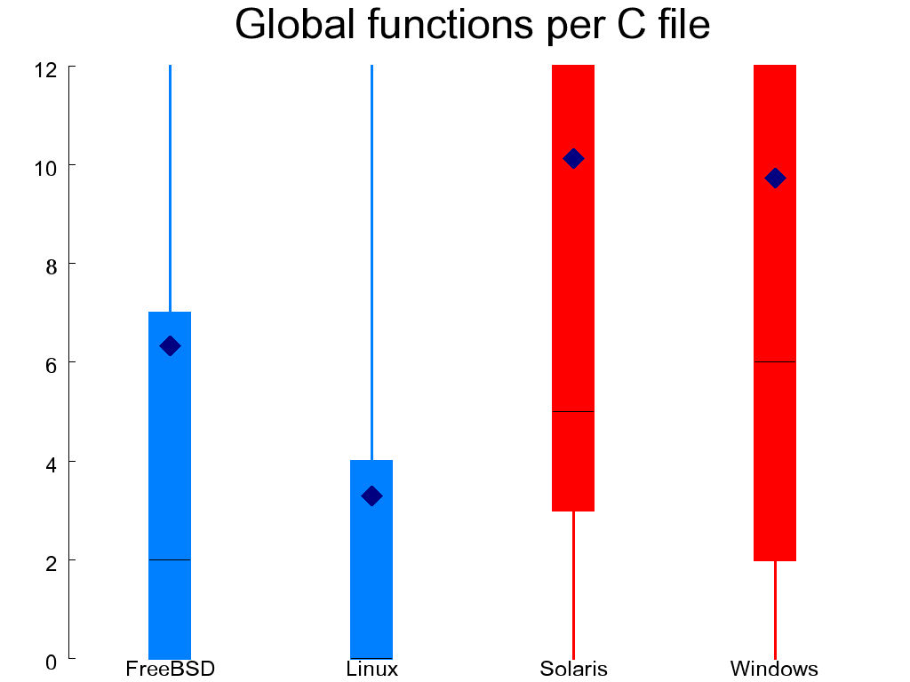
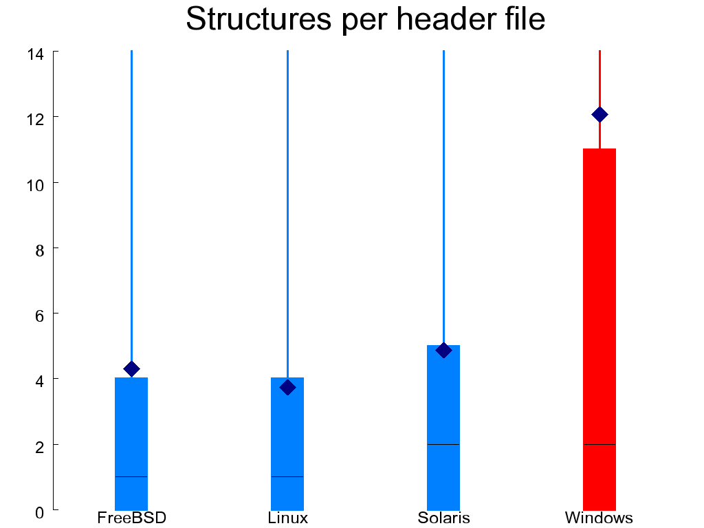
A related measure examines the contents of files, not in terms of lines, but in terms of defined entities. In C source files I count global functions. In header files an important entity is a structure; the closest abstraction to a class that is available in C. Figure 1.4, “Defined global functions (left) and structures (right)” shows the number of global functions that are declared in each C file and the number of aggregates (structures or unions) that are defined in each header file. Ideally, both numbers should be small, indicating an appropriate separation of concerns. The C files of OpenSolaris and WRK come out worse than the other systems, while a significant number of WRK's header files look bad, because they define more than 10 structures each.
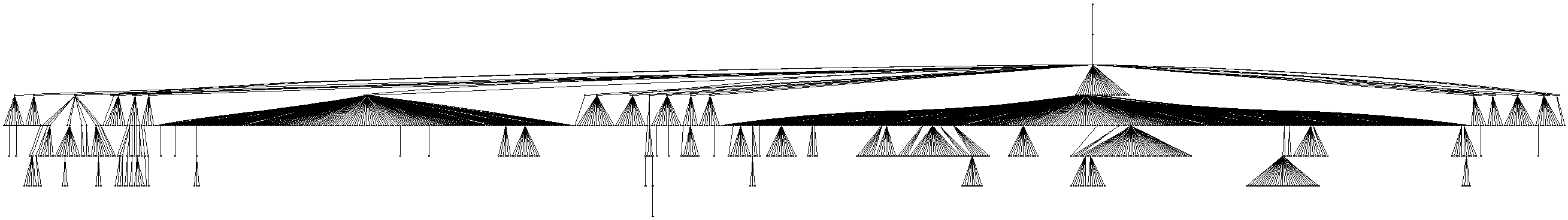
The four systems I've examined have interesting directory structures. As you can see in Figure 1.5, “The directory structure of FreeBSD” to Figure 1.8, “The directory structure of the Windows Research Kernel”, three of the four systems have similarly wide structures. The small size and complexity of the WRK reflects the fact that Microsoft has excluded from it many large parts of the Windows kernel. We see that the directories in Linux are relatively evenly distributed across the whole source code tree, whereas in FreeBSD and OpenSolaris some directories lump together in clusters. This can be the result of organic growth over a longer period of time, because both systems have twenty more years of history on their back (Figure 1.1, “History and geneology of the four systems”). The more even distribution of Linux's directories may also reflect the decentralized nature of its development.


At a higher level of granularity, I examine the number of files located in a single directory. Again, putting many files in a directory is like having many elements in a module. A large number of files can confuse developers, who often search through these files as a group with tools like grep, and lead to accidental identifier collisions through shared header files. The numbers I found in the examined systems can be seen in Table 1.2, “File organization metrics”, and show Linux lagging the other systems.
The next line in the table describes the ratio between header files and C files. I used the following SQL query to calculate these numbers.
select (select count(*) from FILES where name like '%.c') /
 (select count(*) from FILES where name like '%.h')
A common style guideline for C code involves putting each module's interface in a separate header file and its implementation in a corresponding C file. Thus a ratio of header to C files around 1 is the optimum; numbers significantly diverging from one may indicate an unclear distinction between interface and implementation. This can be acceptable for a small system (the ratio in the implementation of the awk programming language is 3/11), but will be a problem in a system consisting of thousands of files. All the systems score acceptably in this metric.
Finally, the last line in Table 1.2, “File organization metrics”
provides a metric related to the complexity of file relationships.
I study this by looking at files as nodes in a directed graph.
I define a file's fan-out as the number of efferent (outgoing)
references it makes to elements declared or defined in other files.
For instance, a C file
that uses the symbols FILE, putc,
and malloc (defined outside the C file in the stdio.h and
stdlib.h header files) has a fan-out of 3.
Correspondingly, I define as a file's fan-in the number
of afferent (incoming) references made by other files.
Thus, in the previous example, the fan-in of stdio.h
would be 2.
I used Henry and Kafura's information flow metric [Henry and Kafura 1981]
to look at the corresponding relationships between files.
The value I report is
(fanIn × fanOut)2
I calculated the value based on the contents of the CScout database
table INCTRIGGERS,
which stores data about symbols in each file that are linked with other files.
select avg(pow(fanout.c * fanin.c, 2)) from
 (select basefileid fid, count(definerid) c from
   (select distinct BASEFILEID, DEFINERID, FOFFSET from INCTRIGGERS) i2 group by basefileid) fanout
 inner join
 (select definerid fid, count(basefileid) c from
   (select distinct BASEFILEID, DEFINERID, FOFFSET from INCTRIGGERS) i2 group by definerid) fanin
 on fanout.fid = fanin.fid
The calculation works as follows.
For the connections each file makes the innermost select
statements derive a set of unique identifiers and the files they are defined or referenced.
Then, the middle select statements count the number of identifiers per file, and the
outermost select statement joins each file's definitions with its references
and calculates the corresponding information flow metric.
A large value for this metric has been associated with the
occurrence of changes and structural flaws.
Table 1.3. Code structure metrics
| Metric | Ideal | FreeBSD | Linux | Solaris | WRK |
|---|---|---|---|---|---|
| % global functions | ↓ | 36.7 | 21.2 | 45.9 | 99.8 |
| % strictly structured functions | ↑ | 27.1 | 68.4 | 65.8 | 72.1 |
| % labeled statements | ↓ | 0.64 | 0.93 | 0.44 | 0.28 |
| Average number of parameters to functions | ↓ | 2.08 | 1.97 | 2.20 | 2.13 |
| Average depth of maximum nesting | ↓ | 0.86 | 0.88 | 1.06 | 1.16 |
| Tokens per statement | ↓ | 9.14 | 9.07 | 9.19 | 8.44 |
| % of tokens in replicated code | ↓ | 4.68 | 4.60 | 3.00 | 3.81 |
| Average structure complexity in functions | ↓ | 7.1 ×10⁴ | 1.3 ×10⁸ | 3.0 ×10⁶ | 6.6 ×10⁵ |
The code structures of the four systems illustrates how similar problems can be tackled through different control structures and separation of concerns. It also allows us to peer into the design of each system.
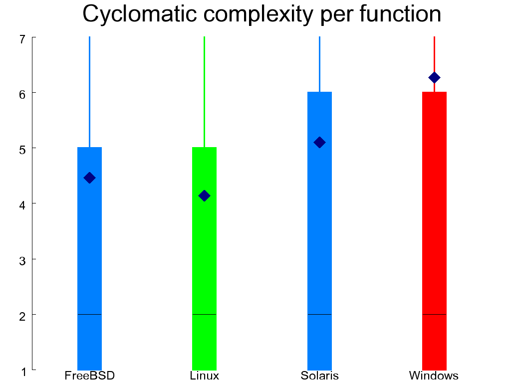
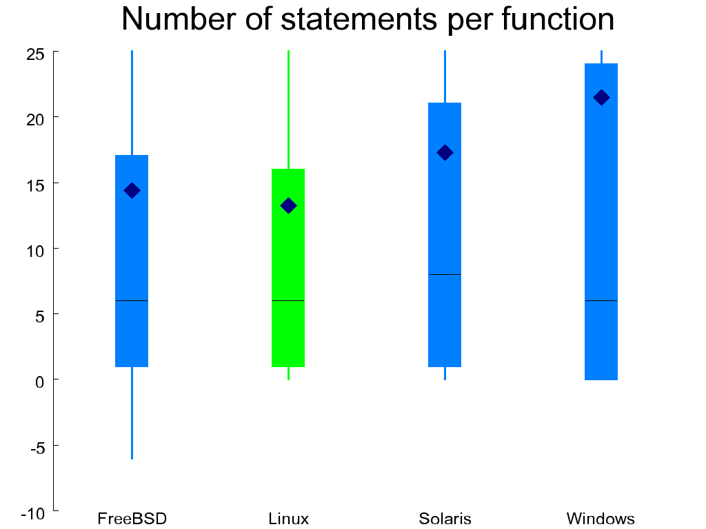
Figure 1.9, “Extended cyclomatic complexity (left) and number of statements per function (right)” shows the distribution across functions of the extended cyclomatic complexity metric [McCabe 1976]. This is a measure of the number of independent paths contained in each function. The number shown takes into account Boolean and conditional evaluation operators (because these introduce additional paths), but not multi-way switch statements, because these would disproportionally affect the result for code that is typically cookie-cutter similar. The metric was designed to measure a program's testability, understandability, and maintainability [Gill and Kemerer 1991]. In this regard Linux scores better than the other systems and the WRK worse. The same figure also shows the number of C statements per function. Ideally, this should be a small number (e.g. around 20) allowing the function's complete code to fit on the developer's screen. Linux again scores better than the other systems.
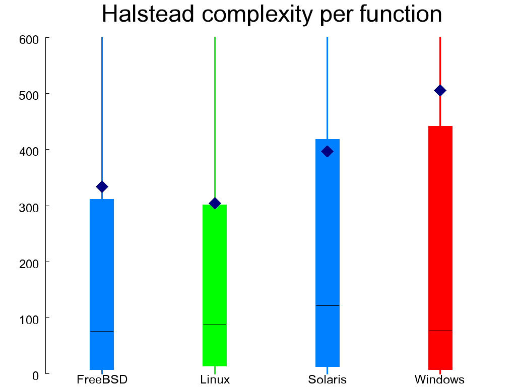
In Figure 1.10, “Halstead complexity per function” we can see the distribution of the Halstead volume complexity [Halstead 1977]. For a given piece of code this is based on four numbers.
- n1
Number of distinct operators
- n2
Number of distinct operands
- N1
Total number of operators
- N2
Total number of operands
Given these four numbers we calculate the program's so-called volume as
(N1 + N2) × log2(n1 + n2)
For instance, for the expression
op = &(!x ? (!y ? upleft : (y == bottom ? lowleft : left)) :
(x == last ? (!y ? upright : (y == bottom ? lowright : right)) :
(!y ? upper : (y == bottom ? lower : normal))))[w->orientation];
the four variables have the following values.
- n1
= & () ! ?: == [] ->(8)- n2
bottom last left lower lowleft lowright normal op orientation right upleft upper upright w x y(16)- N1
27
- N2
24
The theory behind calculating the Halstead volume complexity number is that it should be low, reflecting code that doesn't require a lot of mental effort to comprehend. This metric, however, has often been criticized. As was the case with the cyclomatic complexity, Linux scores better and the WRK worse than the other systems.
Taking a step back to look at interactions between functions,
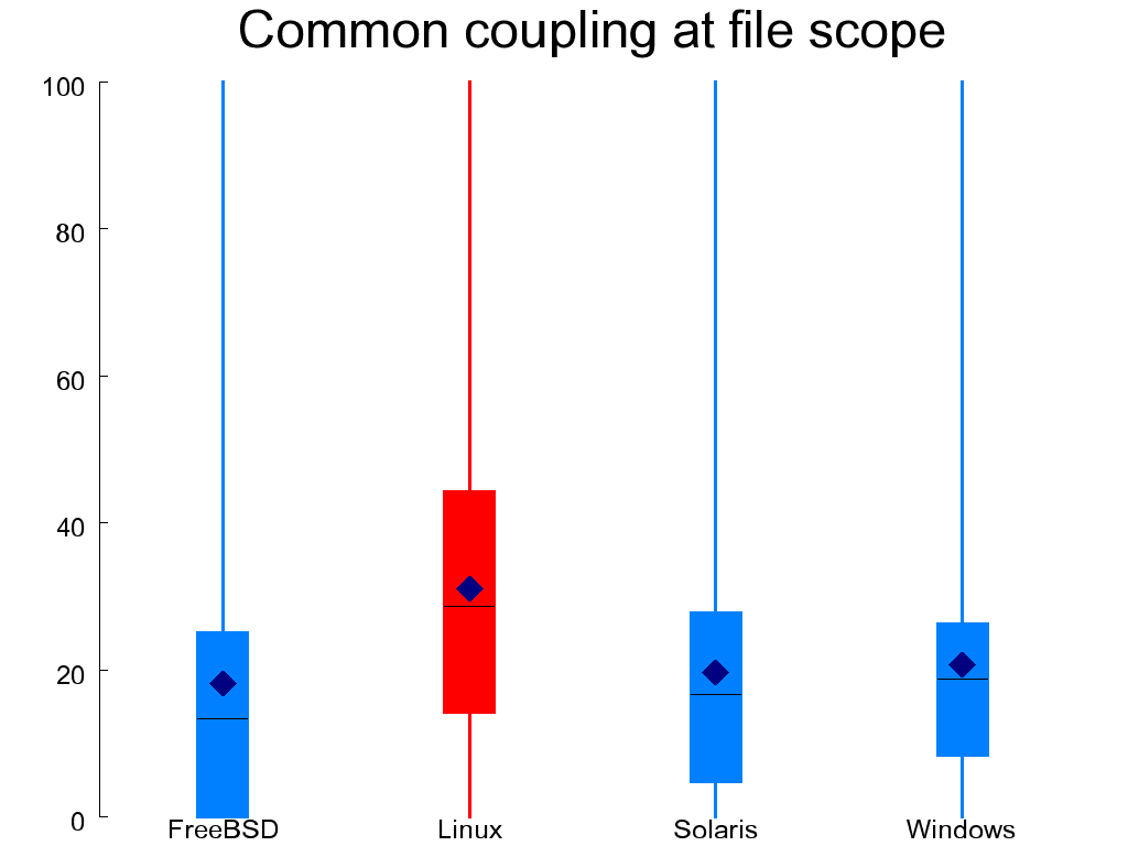
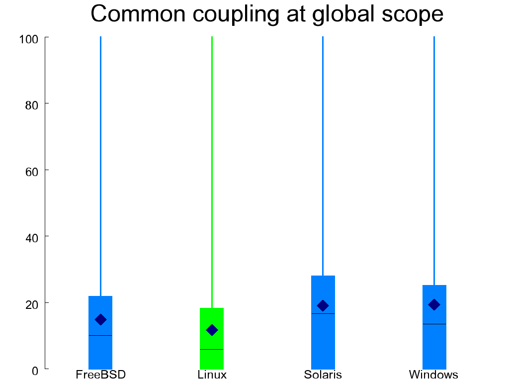
Figure 1.11, “Common coupling at file (left) and global (right) scope” depicts common coupling in functions
by showing the percentage of the unique identifiers appearing in
a function's body that come either from the scope of the compilation
unit (file-scoped identifiers declared as static) or from the project scope (global objects).
Both forms of coupling are undesirable, with the
global identifiers considered worse than the file-scoped ones.
Linux scores better than the other systems in the case of common coupling at the global scope,
but (probably because of this) scores worse than them when looking at the file scope.
All other systems are more evenly balanced.
Other metrics associated with code structure appear in Table 1.3, “Code structure metrics”. The percentage of global functions indicates the functions visible throughout the system. The number of such functions in the WRK (nearly 100%; also verified by hand) is shockingly high. It may however reflect Microsoft's use of different techniques—such as linking into shared libraries (DLLs) with explicitly exported symbols—for avoiding identifier clashes.
Strictly structured functions are those following the rules
of structured programming:
a single point of exit and no goto statements.
The simplicity of such functions makes it easier to reason about them.
Their percentage is calculated by looking at the number of keywords
within each function through the following SQL query.
select 100 -
(select count(*) from FUNCTIONMETRICS where nreturn > 1 or ngoto > 0) /
(select count(*) from FUNCTIONMETRICS) * 100
Along the same lines, the percentage of labeled
statements indicates goto targets:
a severe violation of structured programming
principles.
I measured labeled statements rather than goto
statements, because many branch targets are a lot
more confusing than many branch sources.
Often multiple goto statements to a single
label are used to exit from a function while performing
some cleanup—the equivalent of an exception's finally
clause.
The number of arguments to a function is an indicator of the interface's quality: when many arguments must be passed, packaging them into a single structure reduces clutter and opens up opportunities for optimization in style and performance.
Two metrics tracking the code's understandability are the average depth of maximum nesting and the number of tokens per statement. These metrics are based on the theories that both deeply nested structures and long statements are difficult to comprehend [Cant et al. 1995].
Replicated code has been associated with bugs [Li et al. 2006] and maintainability problems [Spinellis 2006]. The corresponding metric (% of tokens in replicated code) shows the percentage of the code's tokens that participate in at least one clone set. To obtain this metric I used the CCFinderX[3] tool to locate the duplicated code lines and a script (Example 1.1, “Determining the percentage of code duplication from the CCFinderX report”) to measure the ratio of such lines.
Example 1.1. Determining the percentage of code duplication from the CCFinderX report
# Process CCFinderX results
open(IN, "ccfx.exe P $ARGV[0].ccfxd|") || die;
while (<IN>) {
	chop;
	if (/^source_files/ .. /^\}/) {
		# Process file definition lines like the following:
		# 611     /src/sys/amd64/pci/pci_bus.c        1041
		($id, $name, $tok) = split;
		$file[$id][$tok - 1] = 0 if ($tok > 0);
		$nfile++;
	} elsif (/^clone_pairs/ .. /^\}/) {
		# Process pair identification lines like the following for files 14 and 363:
		# 1908    14.1753-1832    363.1909-1988
		($id, $c1, $c2) = split;
		mapfile($c1);
		mapfile($c2);
	}
}

# Add up and report tokens and cloned tokens
for ($fid = 0; $fid <= $#file; $fid++) {
	for ($tokid = 0; $tokid <= $#{$file[$fid]}; $tokid++) {
		$ntok++;
		$nclone += $file[$fid][$tokid];
	}
}
print "$ARGV[0] nfiles=$nfile ntok=$ntok nclone=$nclone ", $nclone / $ntok * 100, "\n";

# Set the file's cloned lines to 1
sub mapfile
{
	my($clone) = @_;
	my ($fid, $start, $end) = ($clone =~ m/^(\d+)\.(\d+)\-(\d+)$/);
	for ($i = $start; $i <= $end; $i++) {
		$file[$id][$i] = 1;
	}
}
Finally, the average structure complexity in functions uses Henry and Kafura's information flow metric [Henry and Kafura 1981] again to look at the relationships between functions. Ideally we would want this number to be low, indicating an appropriate separation between suppliers and consumers of functionality.
Table 1.4. Code style metrics
| Metric | Ideal | FreeBSD | Linux | Solaris | WRK |
|---|---|---|---|---|---|
| % style conforming lines | ↑ | 77.27 | 77.96 | 84.32 | 33.30 |
| % style conforming typedef identifiers | ↑ | 57.1 | 59.2 | 86.9 | 100.0 |
| % style conforming aggregate tags | ↑ | 0.0 | 0.0 | 20.7 | 98.2 |
| Characters per line | ↓ | 30.8 | 29.4 | 27.2 | 28.6 |
| % of numeric constants in operands | ↓ | 10.6 | 13.3 | 7.7 | 7.7 |
| % unsafe function-like macros | ↓ | 3.99 | 4.44 | 9.79 | 4.04 |
| % misspelled comment words | ↓ | 33.0 | 31.5 | 46.4 | 10.1 |
| % unique misspelled comment words | ↓ | 6.33 | 6.16 | 5.76 | 3.23 |
Various choices of indentation, spacing, identifier names, representations for constants, and naming conventions can distinguish sets of code that functionally do exactly the same thing. [Kernighan and Plauger 1978], [The FreeBSD Project 1995], [Cannon et al.], [Stallman et al. 2005]. In most sane cases, consistency is more important than the specific code style convention that was chosen.
For this study, I measured each system's consistency of style by applying the formatting program indent[4] on the complete source code of each system, and counting the lines that indent modified. The result appears on the first line of Table 1.4, “Code style metrics”. The behavior of indent can be modified using various options in order to match a formatting style's guidelines. For instance, one can specify the amount of indentation and the placement of braces. In order to determine each system's formatting style and use the appropriate formatting options, I first run indent on each system with various values of the 15 numerical flags, and turning on or off each one of the 55 Boolean flags (see Example 1.2, “Determining a system's indent formatting options (Unix variants)” and Example 1.3, “Determining a system's indent formatting options (Windows)”). I then chose the set of flags that produced the largest number of conforming lines. For example, on the OpenSolaris source code indent with its default flags would reformat 74% of the lines. This number shrank to 16% once the appropriate flags were determined (-i8 -bli0 -cbi0 -ci4 -ip0 -bad -bbb -br -brs -ce -nbbo -ncs -nlp -npcs).
Example 1.2. Determining a system's indent formatting options (Unix variants)
DIR=$1
NFILES=0
RNFILES=0

# Determine the files that are OK for indent
for f in `find $DIR -name '*.c'`
do
	# The error code is not always correct, so we have to grep for errors
	if indent -st $f 2>&1 >/dev/null | grep -q Error:
	then
		REJECTED="$REJECTED $f"
		RNFILES=`expr $RNFILES + 1`
		echo -n "Rejecting $f - number of lines: "
		wc -l <$f
	else
		FILES="$FILES $f"
		NFILES=`expr $NFILES + 1`
	fi
done

LINES=`echo $FILES | xargs cat | wc -l`
RLINES=`echo $REJECTED | xargs cat | wc -l`

# Format the files with the specified options
# Return the number of mismatched lines
try()
{
	for f in $FILES
	do
		indent -st $IOPT $1 $f |
		diff $f -
	done |
	grep '^<' |
	wc -l
}

# Report the results in a format suitable for further processing
status()
{
	echo "$IOPT: $VIOLATIONS violations in $LINES lines of $NFILES files ($RLINES of $RNFILES files not processed)"
}

# Determine base case
VIOLATIONS=`try`
status
Example 1.3. Determining a system's indent formatting options (Windows)
# Try various numerical options with values 0-8
for try_opt in i ts bli c cbi cd ci cli cp d di ip l lc pi
do
	BEST=$VIOLATIONS
	for n in 0 1 2 3 4 5 6 7 8
	do
		NEW=`try -$try_opt$n`
		if [ $NEW -lt $BEST ]
		then
			BNUM=$n
			BEST=$NEW
		fi
	done
	if [ $BEST -lt $VIOLATIONS ]
	then
		IOPT="$IOPT -$try_opt$BNUM"
		VIOLATIONS=$BEST
		status
	fi
done

# Try the various Boolean options
for try_opt in bad bap bbb bbo bc bl bls br brs bs cdb cdw ce cs bfda \
    bfde fc1 fca hnl lp lps nbad nbap nbbo nbc nbfda ncdb ncdw nce \
    ncs nfc1 nfca nhnl nip nlp npcs nprs npsl nsaf nsai nsaw nsc nsob \
    nss nut pcs prs psl saf sai saw sc sob ss ut
do
	NEW=`try -$try_opt`
	if [ $NEW -lt $VIOLATIONS ]
	then
		IOPT="$IOPT -$try_opt"
		VIOLATIONS=$NEW
	fi
	status
done
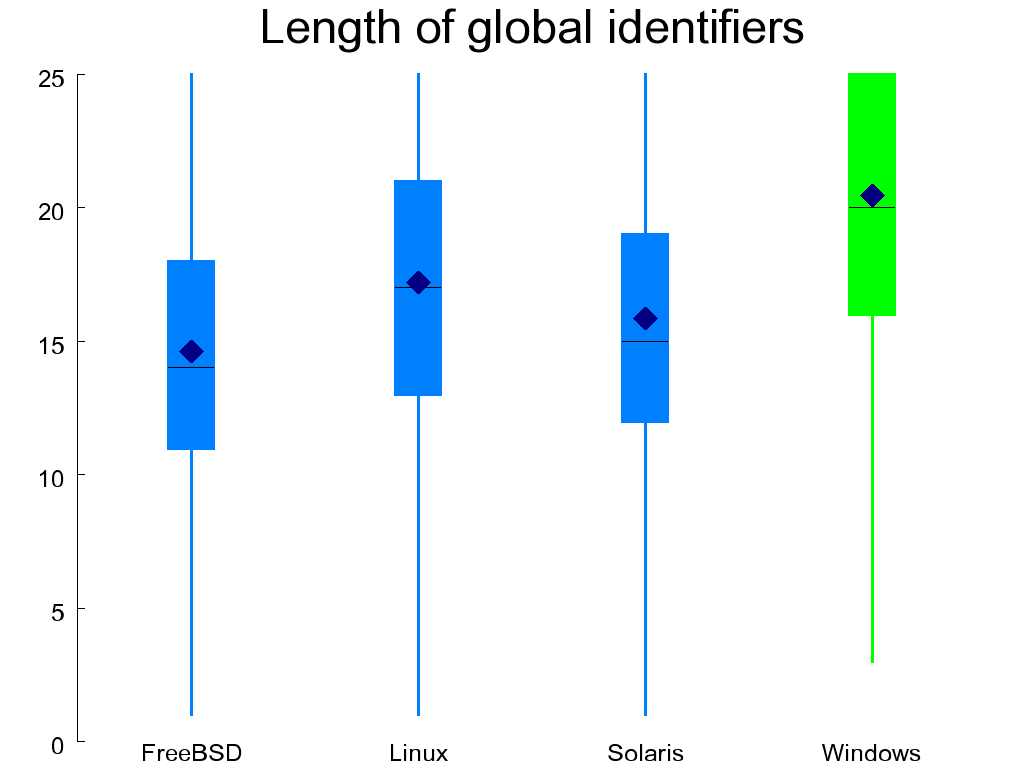
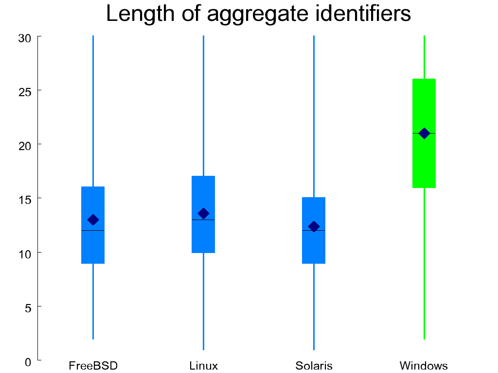
Figure 1.12, “Length of global (left) and aggregate (right) identifiers” depicts the length distribution of two important classes of C identifiers: those of globally visible objects (variables and functions) and the tags used for identifying aggregates (structures and unions). Because each class typically uses a single name space, it is important to choose distinct and recognizable names (see chapter 31 of reference [McConnell 2004]). For these classes of identifiers, longer names are preferable, and the WRK excels in both cases, as anyone who has programmed using the Windows API could easily guess.
Some other metrics related to code style appear in Table 1.4, “Code style metrics”.
To measure consistency, I also determined through code inspection the convention used for naming typedefs
and aggregate tags, and then counted the identifiers of those
classes that did not match the convention.
Here are the two SQL queries I ran, one on the Unix-like systems and
the other on the WRK.
select 100 * (select count(*) from IDS where typedef and name like '%_t') /
  (select count(*) from IDS where typedef)

select 100 * (select count(*) from IDS where typedef and name regexp '^[A-Z0-9_]*$') /
  (select count(*) from IDS where typedef)
Three other metrics aimed at identifying programming practices that style guidelines typically discourage:
Overly long lines of code (characters per line metric)
The direct use of “magic” numbers in the code (% of numeric constants in operands),
The definition of function-like macros that can misbehave when placed after an
ifstatement (% unsafe function-like macros)[5]
The following SQL query roughly calculates the percentage
of unsafe function-like macros by looking for bodies of such
macros that contain more than one statement, but no do keywords.
The result represents a lower bound, because the query can miss other
unsafe macros, such as those consisting of an if statement.
select 100.0 * (select count(*) from FUNCTIONMETRICS left join
  FUNCTIONS on functionid = id where defined and ismacro and ndo = 0 and nstmt > 1) /
(select count(*) from FUNCTIONS where defined and ismacro)
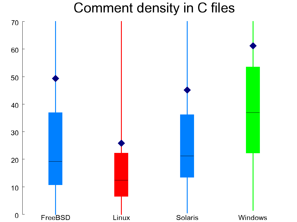
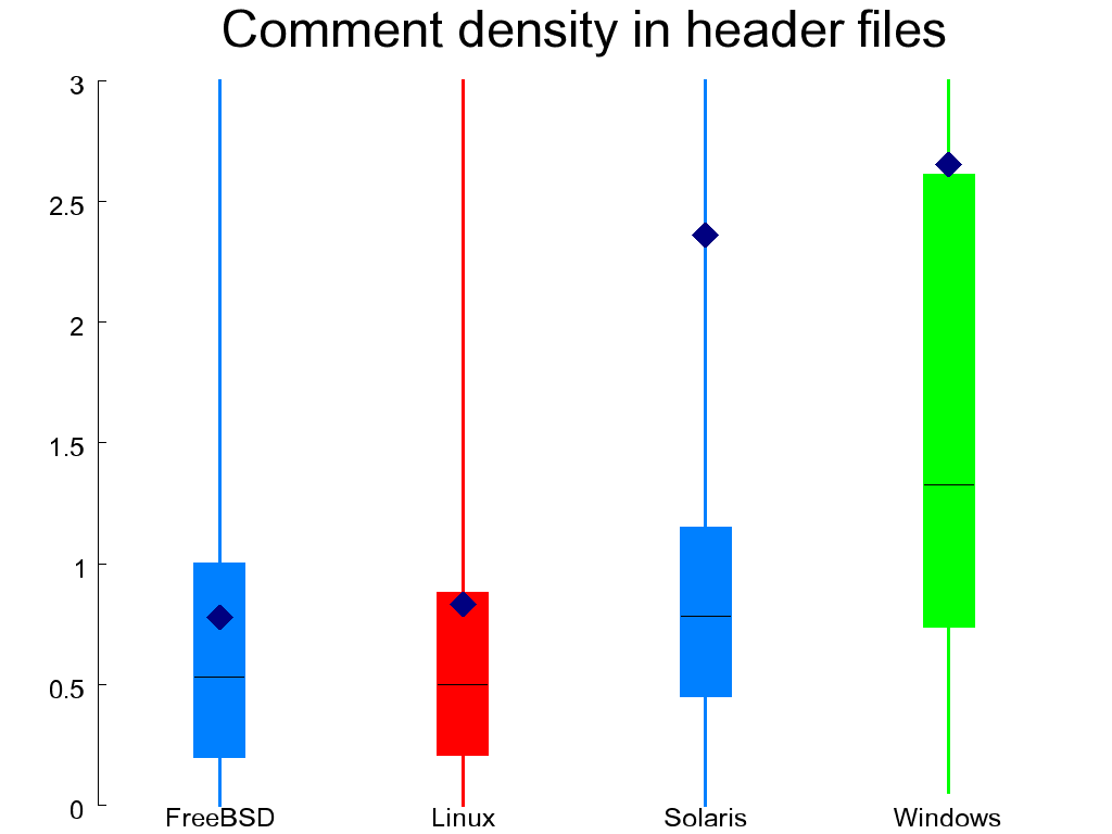
Another important element of style involves commenting. It is difficult to judge objectively the quality of code comments. Comments can be superfluous or even wrong. We can't programmatically judge quality on that level, but we can easily measure the comment density. So Figure 1.13, “Comment density in C (left) and header (right) files” shows the the comment density in C files as the ratio of comment characters to statements. In header files I measured it as the ratio of defined elements that typically require an explanatory comment (enumerations, aggregates and their members, variable declarations, and function-like macros) to the number of comments. In both cases I excluded files with trivially little content. With remarkable consistency, the WRK scores better than the other systems in this regard and Linux worse. Interestingly, the mean value of comment density is a lot higher than the median, indicating that some files require substantially more commenting than others.
select nccomment / nstatement from FILES where name like '%.c' and nstatement > 0

select (nlcomment + nbcomment) / (naggregate + namember + nppfmacro + nppomacro + nenum +
  npfunction + nffunction + npvar + nfvar)
  from FILES
  where name like '%.h' and naggregate + namember + nppfmacro + nppomacro > 0 and nuline / nline < .2
I also measured the number of spelling errors in the comments as a proxy for their quality. For this I ran the text of the comments through the aspell spelling checker with a custom dictionary consisting of all the system's identifier and file names (see Example 1.4, “Counting comment words and misspelings in a CScout database”). The low number of errors in the WRK reflects the explicit spell-checking that according to accompanying documentation, was performed before the code was released.
Example 1.4. Counting comment words and misspelings in a CScout database
# Create personal dictionary of correct words
# from identifier names appearing in the code
PERS=$1.en.pws
(
echo personal_ws-1.1 en 0
	(
	mysql -e 'select name from IDS union select name from FUNCTIONS union select name from FILES' $1 |
	tr /._ \\n |
	sed 's/\([a-z]\)\([A-Z]\)/\1\
\2/g'
	mysql -e 'select name from IDS union select name from FUNCTIONS union select name from FILES' $1 |
	tr /. \\n
	) |
sort -u
) >$PERS

# Get comments from source code files and spell check them
mysql -e 'select comment from COMMENTS left join FILES on COMMENTS.FID = FILES.FID where not name like "%.cs"' $1 |
sed 's/\\[ntrb]//g' |
tee $1.comments |
aspell --lang=en --personal=$PERS -C --ignore=3 --ignore-case=true  --run-together-limit=10 list >$1.err
wc -w $1.comments	# Number of words
wc -l $1.err		# Number of errors
Although I did not measure portability objectively, the work involved
in processing the source code with CScout allowed me to get a feeling
of the portability of each system's source code between different compilers.
The code of Linux and WRK appears to be the one most tightly bound
to a specific compiler.
Linux uses numerous language extensions provided by the GNU
C compiler, sometimes including assembly code thinly disguised
in what passes as C syntax in gcc
(see Figure 1.14, “The definition of memmove in the Linux kernel”).
The WRK uses considerably fewer language extensions, but
relies significantly on the try catch extension to
C that the Microsoft compiler supports.
The FreeBSD kernel uses only a few gcc extensions, and these
are often isolated inside wrapping macros.
The OpenSolaris kernel was a welcome surprise:
it was the only body of source code that did not require any
extensions to CScout in order to compile.
Figure 1.14. The definition of memmove in the Linux kernel
void *memmove(void *dest, const void *src, size_t n)
{
        int d0, d1, d2;

        if (dest < src) {
                memcpy(dest,src,n);
        } else {
                __asm__ __volatile__(
                        "std\n\t"
                        "rep\n\t"
                        "movsb\n\t"
                        "cld"
                        : "=&c" (d0), "=&S" (d1), "=&D" (d2)
                        :"0" (n),
                         "1" (n-1+(const char *)src),
                         "2" (n-1+(char *)dest)
                        :"memory");
        }
        return dest;
}
Table 1.5. Preprocessing metrics
| Metric | Ideal | FreeBSD | Linux | Solaris | WRK |
|---|---|---|---|---|---|
| % of preprocessor directives in header files | ↓ | 22.4 | 21.9 | 21.6 | 10.8 |
| % of non-#include directives in C files | ↓ | 2.2 | 1.9 | 1.2 | 1.7 |
| % of preprocessor directives in functions | ↓ | 1.56 | 0.85 | 0.75 | 1.07 |
| % of preprocessor conditionals in functions | ↓ | 0.68 | 0.38 | 0.34 | 0.48 |
| % of function-like macros in defined functions | ↓ | 26 | 20 | 25 | 64 |
| % of macros in unique identifiers | ↓ | 66 | 50 | 24 | 25 |
| % of macros in identifiers | ↓ | 32.5 | 26.7 | 22.0 | 27.1 |
The relationship between the C language proper and its (integral) preprocessor can at best be described as uneasy. Although C and real-life programs rely significantly on the preprocessor, its features often create portability, maintainability, and reliability problems. The preprocessor, as a powerful but blunt instrument, wrecks havoc with identifier scopes, the ability to parse and refactor unpreprocessed code, and the way code is compiled on different platforms. Thus most C programming guidelines recommend moderation in the use of preprocessor constructs. Also for this reason modern languages based on C have tried to replace features provided by the C preprocessor with more disciplined alternatives. For instance, C++ provides constants and powerful templates as alternatives to the C macros, while C# provides preprocessor-like functionality only to aid conditional compilation and code generators.
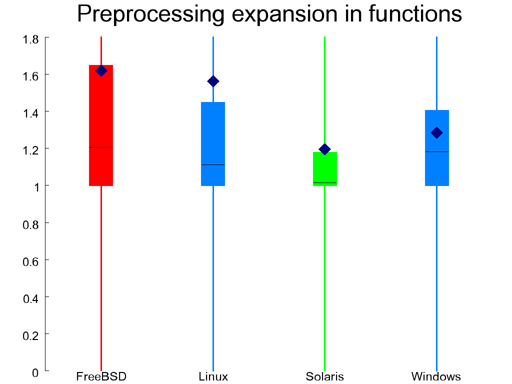
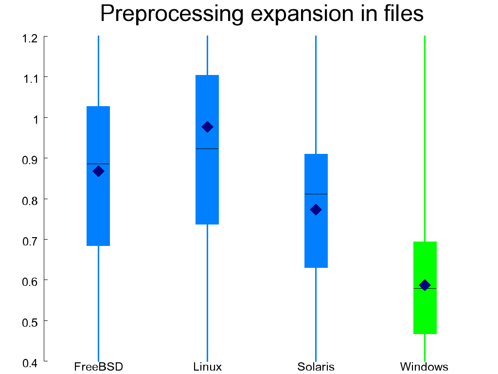
The use of preprocessor features can be measured by the amount of expansion or contraction that occurs when the preprocessor runs over the code. Figure 1.15, “Preprocessing expansion in functions (left) and files (right)” contains two such measures: one for the body of functions (representing expansion of code), and one for elements outside the body of functions (representing data definitions and declarations). The two measurements were made by calculating the ratio of tokens arriving into the preprocessor to those coming out of it. Here is the SQL query I used for calculating the expansion of code inside functions.
select nctoken / npptoken from FUNCTIONS
inner join FUNCTIONMETRICS on id = functionid
where defined and not ismacro and npptoken > 0
Both expansion and contraction are worrisome: expansion signifies the occurrence of complex macros, while contraction is a sign of conditional compilation, which is also considered harmful [Spencer and Collyer 1992]. Therefore, the values of these metrics should hover around 1. In the case of functions OpenSolaris scores better than the other systems and FreeBSD worse, while in the case of files the WRK scores substantially worse than all other systems.
Four further metrics listed in Table 1.5, “Preprocessing metrics” measure increasingly unsafe uses of the preprocessor:
Directives in header files (often required)
Non-
#includedirectives in C files (rarely needed)Preprocessor directives in functions (of dubious value)
Preprocessor conditionals in functions (a portability risk)
Preprocessor macros are typically used instead of variables (where we call these macros object-like macros) and functions (where we call them function-like macros). In modern C, object-like macros can often be replaced through enumeration members and function-like macros through inline functions. Both alternatives adhere to the scoping rules of C blocks and are therefore considerably safer than macros, whose scope typically spans a whole compilation unit. The last three metrics of preprocessor use in Table 1.5, “Preprocessing metrics” measure the occurrence of function-like and object-like macros. Given the availability of viable alternatives and the dangers associated with macros, all should ideally have low values.
Table 1.6. Data organization metrics
| Metric | Ideal | FreeBSD | Linux | Solaris | WRK |
|---|---|---|---|---|---|
| % of variable declarations with global scope | ↓ | 0.36 | 0.19 | 1.02 | 1.86 |
| % of variable operands with global scope | ↓ | 3.3 | 0.5 | 1.3 | 2.3 |
| % of identifiers with wrongly global scope | ↓ | 0.28 | 0.17 | 1.51 | 3.53 |
| % of variable declarations with file scope | ↓ | 2.4 | 4.0 | 4.5 | 6.4 |
| % of variable operands with file scope | ↓ | 10.0 | 6.1 | 12.7 | 16.7 |
| Variables per typedef or aggregate | ↓ | 15.13 | 25.90 | 15.49 | 7.70 |
| Data elements per aggregate or enumeration | ↓ | 8.5 | 10.0 | 8.6 | 7.3 |
The final set of measurements concerns the organization of each kernel's (in-memory) data. A measure of the quality of this organization in C code can be determined by the scoping of identifiers and the use of structures.
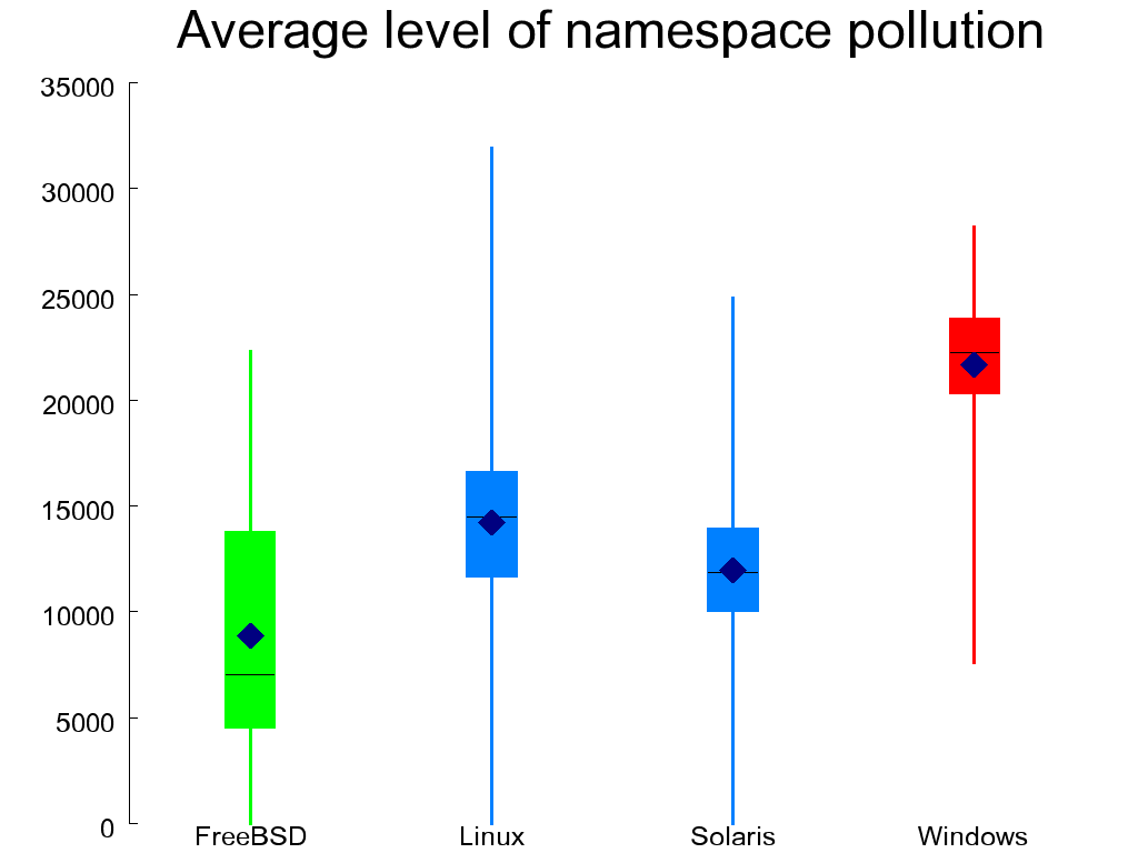
In contrast to many modern languages, C provides few mechanisms for controlling namespace pollution. Functions can be defined in only two possible scopes (file and global), macros are visible throughout the compilation unit in which they are defined, and aggregate tags typically live all together in the global namespace. For the sake of maintainability, it's important for large-scale systems such as the four examined in this chapter to judiciously use the few mechanisms available to control the large number of identifiers that can clash.
Figure 1.16, “Average level of namespace pollution in C files” shows the level of namespace pollution in C files by averaging the number of identifiers and macros that are visible at the start of each function. With roughly 10,000 identifiers visible on average at any given point across the systems I examine, it is obvious that namespace pollution is a problem in C code. Nevertheless, FreeBSD fares better than the other systems and the WRK worse.
The first three measures in Table 1.6, “Data organization metrics” examine how each system deals with its scarcest naming resource, global variable identifiers. One would like to minimize the number of variable declarations that take place at the global scope in order to minimize namespace pollution. Furthermore, minimizing the percentage of operands that refer to global variables reduces coupling and lessens the cognitive load on the reader of the code (global identifiers can be declared anywhere in the millions of lines comprising the system). The last metric concerning global objects counts identifiers that are declared as global, but could have been declared with a static scope, because they are accessed only within a single file. The corresponding SQL query calculates the percentage of identifiers with global (linkage unit) scope that exist only in a single file.
select 100.0 * (select count(*) from
  (select  TOKENS.eid from TOKENS
    left join IDS on TOKENS.eid = IDS.eid
    where ordinary and lscope group by eid having min(fid) = max(fid) ) static) /
  (select count(*) from IDS)
The next two metrics look at variable declarations and operands with file scope. These are more benign than global variables, but still worse than variables scoped at a block level.
The last two metrics concerning the organization of data provide a crude measure of the abstraction mechanisms used in the code. Type and aggregate definitions are the two main data abstraction mechanisms available to C programs. Therefore, counting the number of variable declarations that correspond to each type or aggregate definition provides an indication of how much these abstraction mechanisms have been employed.
select ((select count(*) from IDS where ordinary and not fun) /
  (select count(*) from IDS where suetag or typedef))

select ((select count(*) from IDS where sumember or enum)  /
  (select count(*) from IDS where suetag))
These statements measure the number of data elements per aggregate or enumeration in relation to data elements as a whole. This is similar to the relation that Chidamber and Kemerer's object-oriented weighted methods per class (WMC—[Chidamber and Kemerer 1994])) metric has to code. A high value could indicate that a structure tries to store too many disparate elements.
[5] Function-like
macros containing more than one statement should have their
body enclosed in a dummy do ... while(0) block
in order to make them behave like a call to a real
function.