Large Production Line Optimization Using Simulated Annealing

http://www.spinellis.gr/pubs/jrnl/1999-IJPR-Optim/html/bap.html
This is an HTML rendering of a working paper draft that led to a publication. The publication should always be cited in preference to this draft using the following reference:

Diomidis Spinellis, Chrissoleon Papadopoulos, and Jim MacGregor Smith. Large production line optimization using simulated annealing. International Journal of Production Research, 38(3):509–541, February 2000. (doi:10.1080/002075400189284)

The above paper has been cited 22 times.

This document is also available in PDF format.

The document's metadata is available in BibTeX format.

This material is presented to ensure timely dissemination of scholarly and technical work. Copyright and all rights therein are retained by authors or by other copyright holders. All persons copying this information are expected to adhere to the terms and constraints invoked by each author's copyright. In most cases, these works may not be reposted without the explicit permission of the copyright holder.

Diomidis Spinellis Publications

Large Production Line Optimization Using Simulated Annealing

Diomidis Spinellis
Department of Information and Communication Systems
University of the Aegean
83200 Karlovasi
Samos, Greece.
email: dspin@aegean.gr

Chrissoleon Papadopoulos
Department of Business Administration
University of the Aegean
82100 Chios, Greece
email: hpap@aegean.gr

J. MacGregor Smith
Department of Mechanical and Industrial Engineering
University of Massachusetts
Amherst Massachusetts 01003, USA
email: jmsmith@ecs.umaecs.edu

Abstract

We present a robust generalized queueing network algorithm as an evaluative procedure for optimizing production line configurations using simulated annealing. We compare the results obtained with our algorithm to those of other studies and find some interesting similarities but also striking differences between them in the allocation of buffers, numbers of servers, and their service rates. While context dependent, these patterns of allocation are one of the most important insights which emerge in solving very long production lines. The patterns, however, are often counter-intuitive, which underscores the difficulty of the problem we address. The most interesting feature of our optimization procedure is its bounded execution time, which makes it viable for optimizing very long production line configurations. Based on the bounded execution time property, we have optimized configurations of up to 60 stations with 120 buffers and servers in less than five hours of CPU time.

Keywords: Buffer Allocation, Nonlinear, Stochastic, Integer, Network Design, Simulated Annealing

1 Introduction and Literature Review

A large amount of research has been devoted to the analysis and design of production lines. A lot of this research concerns the design of manufacturing systems with considerable inherent variability in the processing times at the various stations, a common situation with human operators/assemblers. The literature on the modelling and optimization of production lines is vast, allowing us to review only the most directly relevant studies. For a systematic classification of the relevant works on the stochastic modelling of these and other types of manufacturing systems (e.g., transfer lines, flexible manufacturing systems (FMS) and flexible assembly systems (FAS)), the interested reader is referred to a review paper by Papadopoulos and Heavey [63] and some recently published books, such as those by Askin and Standridge [5], Buzacott and Shanthikumar [9], Gershwin [25], Papadopoulos et al. [64], Viswanadham and Narahari [81] and Altiok [2].

Two are the basic problem classes:

the evaluation of production line performance measures such as throughput, mean flow time, workstation mean queue length, and system utilization, and
the optimization of the decision variables of these lines.

Examples of decision variables that have been considered are:

the sizes of the buffers placed between successive workstations of the lines,
the number of servers allocated to each workstation, and
the amount of workload allocated to each workstation.

The corresponding optimization problems are named, respectively, (1) the buffer allocation problem, (2) the server allocation problem and (3) the workload allocation problem, in a production line.

In Papadopoulos et al. [64] both evaluative and generative (optimization) models are given for modelling the various types of manufacturing systems. This work falls into the second category. Evaluative and optimization models can be combined by closing the loop between them; that is, one can use feedback from an evaluative model to modify the decisions taken by the optimization model.

One of the key questions that the designers face in a serial production line is the buffer allocation problem (BAP), i.e., how much buffer storage to allow and where to place it within the line. This is an important question because buffers can have a great impact on the efficiency of the production line. They compensate for the blocking and the starving of the line's stations. For this reason, the buffer allocation problem has received a lot more attention than the other two design problems. Buffer storage is expensive due both to its direct cost, and to the increase of the work-in-process (WIP) inventories. In addition, the requirement to limit the buffer storage can also be a result of space limitations in the shop floor. The literature on the BAP is extensive. A systematic classification of the research work in this area is given in Singh and MacGregor Smith [71] and Papadopoulos et al. [64]. The works are split according to:

The method used to solve the buffer allocation problem: search methods, (Altiok and Stidham [4], MacGregor Smith and Daskalaki [75], Seong et al. [69], and Hillier and So [39] [40]), dynamic programming methods, (Kubat and Sumita [56], Jafari and Shanthikumar [47], and Yamashita and Altiok [83], among others), and simulation methods, (Conway et al. [14]) and Ho et al. [43]).
The type of production line: balanced/unbalanced, (Powell [66] presents a literature review according to this scheme), or reliable/unreliable; the majority of papers deal with reliable lines. Only a few algorithms have been developed to calculate the performance measures of unreliable production lines (Glassey and Hong [26], Choong and Gershwin [13], Gershwin [24], and Heavey, Papadopoulos, and Browne [33]). Hillier and So [39] and Seong, Chang, and Hong [69] have dealt with the buffer allocation problem in unreliable production lines.
The number of machines available at each workstation: Similarly, few researchers have dealt with the buffer allocation problem in production lines with multiple (parallel) machines at each workstation (Hillier and So [41], Magazine and Stecke [60], and Singh and MacGregor Smith [71]).

Apart of the buffer allocation problem, the other two interesting design problems have been also considered by some researchers, e.g., the work allocation problem (Hillier and Boling [37], [34], [36], Ding and Greenberg [19], Huang and Weiss [45], Shanthikumar et al. [70], Wan and Wolff [82] and Yamazaki et al. [84], among others) and the server allocation problem (Magazine and Stecke [60] and Hillier and So [38]). Hillier and So [41] studied various combinations of these three design problems. Other references may be found therein (Buzacott and Shanthikumar [8], [9], among others).

The present work deals with the same design problems (buffer allocation, server allocation and workload allocation) but for long production lines with multi-machine stations.

As the problem being investigated is combinatorial in nature, traditional Operations Researh techniques as not practical for obtaining optimal solutions for long production lines. We propose a simulated annealing (SA) approach as the search method in conjunction with the expansion method developed by Kerbache and MacGregor Smith [50] as the evaluative tool. Simulated annealing is an adaptation of the simulation of physical thermodynamic annealing principles described by Metropolis et al. [61] to the combinatorial optimization problems [53,11]. Similar to genetic algorithms [44,28] and tabu search techniques [27] it follows the ``local improvement'' paradigm for harnessing the exponential complexity of the solution space.

The algorithm is based on randomization techniques. An overview of algorithms based on such techniques can be found in the survey by Gupta et al. [31]. A complete presentation of the method and its applications is described by Van Laarhoven and Aarts [58] and accessible algorithms for its implementation are presented by Corana et al. [15] and Press et al. [67]. A critical evaluation of different approaches to annealing schedules and other method optimizations are given by Ingber [46]. As a tool for operational research SA is presented by Eglese [20], while Koulamas et al. [55] provide a complete survey of SA applications to operations research problems.

The use of the Simulated Annealing algorithm appears to be a promissing approach. We believe that this algorithm could be applied in conjunction with a fast decomposition algorithm to solve efficiently and accurately the aforementioned optimization problems in much longer production lines.

The remainder of the paper is organized as follows: we first describe the production line model and the problem of our interest followed by the methodology of our approach namely: the performance model, the expansion method used for evaluating the line performance, an overview of the combinatorial optimization methods, the simulated annealing optimization method, and the complete enumeration method; we then we describe our experimental methodology and present an overview of the numerical and performance results for short and long production lines. In the Appendix following the concluding section, we provide a full tabulated set of the experimental results.

2 The Production Line Model and the Optimal Design Problem

We define an asynchronous line as one in which every workstation can pass parts on when its processing is complete as long as buffer space is available. Such a line is subject to manufacturing starving and blocking. We assume that the first station is never starved and the last station is never blocked. Therefore we can say that the line operates in a push mode: parts are always available when needed at the first workstation and space is always available at the last workstation to dispose of completed parts.

Figure 1: A N-workstation multi-machine production line with N-1 intermediate buffers

A N-station line consists of N workstations in series, labelled M₁, M₂, Ľ, M_N and N-1 locations for buffers, labelled B₂, B₃, Ľ, B_N, is illustrated in Figure 1. Each station i has s_i servers operating in parallel. The buffer capacities of the intermediate buffers B_i, i = 2,Ľ,N, are denoted by q_i, whereas the mean service times of the i stations (i = 1,Ľ,N) are denoted by w_i.

The main performance measure of the production line is the mean throughput, denoted by R(q,s,w), where q = (q₂,q₃,Ľ,q_N), s = (s₁,s₂,Ľ,s_N) and w = (w₁,w₂,Ľ,w_N).

If Q denotes the total number of available buffer slots to be allocated to the N-1 buffers and S the total number of available servers (machines) to allocated to the N stations then the general version of the optimization model (first reported by Hillier and So, 1995) is:

max

R(q,s,w)

(1)

subject to:

N
ĺ
i = 2

q_i = Q,

(2)

N
ĺ
i = 1

s_i = S,

(3)

N
ĺ
i = 1

w_i = N,

(4)

q_i ł 0 and integer (i = 2,3,Ľ,N),

s_i ł 1 and integer (i = 1,2,Ľ,N),

w_i > 0 (i = 1,2,Ľ,N),

where Q,S and N are fixed constants and q, s and w are the decision vectors. The third constraint indicates that the sum of the expected service times is a fixed constant, which by normalization can be equal to N.

The objective function of throughput, R(q,s,w), is not the only performance measure of interest. The average WIP, the flow time, the cycle time, the system utilization, the average queue lengths and other measures are equally important performance measures. However, throughput is the most commonly used performance measure in the international literature.

3 Optimal Allocation Methodology

3.1 Performance Models

The queueing model M/M/C/K that we use refers to a queueing system where:

it is assumed that the arrivals are distributed according to the Poisson distribution (or equivalently that the intermediate times between two successive arrivals are exponentially distributed),
the service (processing) times follow the exponential distribution,
there are C parallel servers (machines which are identical at each workstation), and
the total capacity of the system is finite and equal to K.

While our focus in this paper is on M/M/C/K approximations for open queueing networks of series-parallel topologies, we also briefly discuss some of the available approaches used for modelling M/M/1/K systems since most of the literature has focused on M/M/1/K systems.

Both open and closed systems have been studied by exact analysis although results have been limited. Exact analyses of open two, three, and four node-server models with exponential service are limited by the explosive growth of the Markov chain models for analyzing these systems. The analysis of very large Markov chain models has led to effective aggregation techniques for these models [68,77] but the computation time and power required for these exact results leaves open the need for approximation techniques.

Van Dijk and his co-authors [79,80] have developed some bounding methodologies for both M/M/1/K and M/M/C/K systems and have demonstrated their usefulness in the design of small queueing networks. Of course, when doing optimization of medium and long queueing networks, bounds can be far off the optimum, so robust approximation techniques close to the optimal performance measures are most desireable.

Most approximation techniques appearing in the literature rely on decomposition/aggregation methods to approximate performance measures. One and two node decompositions of the network have been carried out, all with varying degree of success.

The few approximation approaches available in the literature can be classified as follows: Isolation methods, Repeated Trials, Node-by-node decomposition, and Expansion methods. In the Isolation method, the network is subdivided into smaller subnetworks and then studied in isolation [59,6]. This method was used by Kuehn [57,23] but they failed to consider networks with finite capacity.

Closely related to the Isolation method is the Repeated Trials Method, a class of techniques based upon repeatedly attempting to send blocked customers to a queue causing the blocking [10,22,21].

In Node-by-node decomposition, the network is broken down into single, pairs, and triplets of nodes with augmented service and arrival parameters which are then studied separately [35,78,1,3,65,7]. More general service time approximations appear in [30]. The Expansion method is the approach argued for in this paper for computing the performance measures of M/M/C/K finite queueing networks [49,51,52]. It can be characterized conceptually as a combination of Repeated Trials and Node-by-Node Decomposition where the key difference is that a ``holding'' node is added to the network to register blocked customers. The addition of the holding node ``expands'' the network. This approach transforms the queueing network into an equivalent Jackson network which is then decomposed allowing for each node to be solved independently. We have successfully used the Expansion Method to model M/M/1/K[52], M/M/C/K[48,32], M/G/1/K[51], and most recently M/G/C/C [12,72,73] queues and queueing networks. In addition, we have also used our Expansion Methodology to model routing [18,17,29] and optimal resource allocation problems [75,72,74,71].

3.2 Expansion Method

The Expansion Method is a robust and effective approximation technique developed by Kerbache and Smith [51]. As described in previous papers, this method is characterized as a combination of Repeated Trials and Node-by-node Decomposition solution procedures. Methodologies for computing performance measures for a finite queueing network use primarily the following two kinds of blocking:

Type I:: The upstream node i gets blocked if the service on a customer is completed but it cannot move downstream due to the queue at the downstream node j being full. This is sometimes referred to as Blocking After Service (BAS) [62].
Type II:: The upstream node is blocked when the downstream node becomes saturated and service must be suspended on the upstream customer regardless of whether service is completed or not. This is sometimes referred to as Blocking Before Service (BBS) [62].

The Expansion Method uses Type I blocking, which is prevalent in most production and manufacturing, transportation and other similar systems.

Consider a single node with finite capacity K (including service). This node essentially oscillates between two states - the saturated phase and the unsaturated phase. In the unsaturated phase, node j has at most K- 1 customers (in service or in the queue). On the other hand, when the node is saturated no more customers can join the queue. Refer to Figure 2 for a graphical representation of the two scenarios.

Figure 2: Type I Blocking in Finite Queues

The Expansion Method consists of the following three stages :

Stage I: Network Reconfiguration.
Stage II: Parameter Estimation.
Stage III: Feedback Elimination.

The following notation defined by Kerbache and Smith [51,52] shall be used in further discussion regarding this methodology :

: h: = The holding node established in the Expansion method.
: L := External Poisson arrival rate to the network.
: l_j := Poisson arrival rate to node j.
: [(l_j)\tilde]:= Effective arrival rate to node j.
: m_j := Exponential mean service rate at node j .
: [(m_j)\tilde] := Effective service rate at node j due to blocking.
: p_K:= Blocking probability of finite queue of size K.
: p_K˘:=Feedback blocking probability in the Expansion method.
: p₀^j :=Unconditional probability that there is no customer in the service channel at node j (either being served or being held after service).
: R := Mean throughput rate.
: S_j := Service capacity (buffer) at node j, i.e. S = K for a single queue.

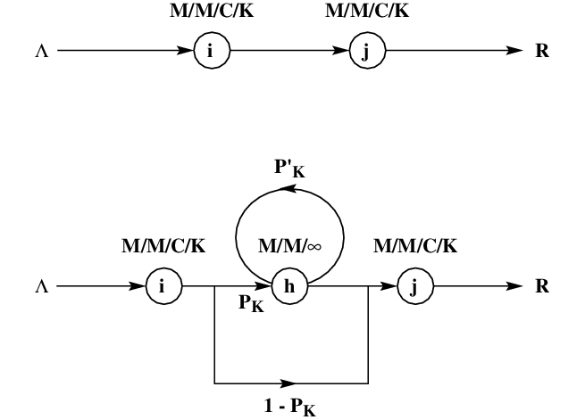
3.2.1 Stage I: Network Reconfiguration

Using the concept of two phases at node j, an artificial node h is added for each finite node in the network to register blocked customers. Figure 2 shows the additional delay, caused to customers trying to join the queue at node j when it is full, with probability p_K. The customers successfully join queue j with a probability (1 - p_K). Introduction of an artificial node also dictates the addition of new arcs with p_K and (1 - p_K) as the routing probabilities.

The blocked customer proceeds to the finite queue with probability (1- p_K˘) once again after incurring a delay at the artificial node. If the queue is still full, it is rerouted with probability p_K˘ to the artificial node where it incurs another delay. This process continues till it finds a space in the finite queue. A feedback arc is used to model the repeated delays. The artificial node is modeled as an M/M/Ą queue. The infinite number of servers is used simply to serve the blocked customer a delay time without queueing.

3.2.2 Stage II: Parameter Estimation

This stage essentially estimates the parameters p_K, p_K˘ and m_h utilizing known results for the M/M/C/K model.

p_K : Analytical results from the M/M/C/K model provide the following expression for p_K.

p_K =

c^K-c c!

ć
ç
č

ö
÷
ř

p₀

(5)

where for (l/cm\not = 1)

p₀ =

é
ę
ë

c-1
ĺ
n = 0

ć
ç
č

ö
÷
ř

(l/m)^c

1 -(l/cm)^K-c+1

1 - l/cm

ů
ú
ű

-1

(6)

and for (l/cm = 1),

p₀ =

é
ę
ë

c-1
ĺ
n = 0

ć
ç
č

ö
÷
ř

(l/m)^c

(K-c + 1)

ů
ú
ű

-1

(7)

p_K˘: Since there is no closed form solution for this quantity an approximation is used given by Labetoulle and Pujolle obtained using diffusion techniques [59].

p_K˘ =

é
ę
ë

m_j + m_h

m_h

l[(r₂^K - r₁^K) - (r₂^K-1 - r₁^K-1)]

m_h[(r₂^K+1 - r₁^K+1) - (r₂^K -r₁^K)]

ů
ú
ű

-1

(8)

where r₁ and r₂ are the roots to the polynomial:

l- (l+ m_h + m_j)x + m_hx² = 0

(9)

while, l = l_j - l_h(1 - p_K˘) and l_j and l_h are the actual arrival rates to the finite and artificial holding nodes respectively.

In fact, l_j the arrival rate to the finite node is given by:

l_j =

~
l_i

(1 - p_K) =

~
l_i

- l_h

(10)

Let us examine the following argument to determine the service time at the artificial node. If an arriving customer is blocked, the queue is full and thus a customer is being serviced, so the arriving customer to the holding node has to remain in service at the artificial holding node for the remaining service time interval of the customer in service. The delay distribution of a blocked customer at the holding node has the same distribution as the remaining service time of the customer being serviced at the node doing the blocking. Using renewal theory, one can show that the remaining service time distribution has the following rate m_h:

m_h =

2m_j

1 + s²m_j²

(11)

where, s² is the service time variance given by Kleinrock [54]. Notice that if the service time distribution at the finite queue doing the blocking is exponential with rate m_j, then:

m_h = m_j

the service time at the artificial node is also exponentially distributed with rate m_j.

3.2.3 Stage III: Feedback Elimination

Due to the feedback loop around the holding node, there are strong dependencies in the arrival processes. Elimination of these dependencies requires reconfiguration of the holding node which is accomplished by recomputing the service time at the node and removing the feedback arc. The new service rate is given by:

m_h˘ = (1 - p_K˘)m_h

(12)

The probabilities of being in any of the two phases (saturated or unsaturated) are p_K and (1 - p_K) . The mean service time at a node i preceding the finite node is m_i^-1 when in the unsaturated phase and (m_i^-1 + m_h˘^-1) in the saturated phase. Thus, on an average, the mean service time at the node i preceding a finite node is given by:

~
m_i^-1

= m_i^-1 + p_Km_h^-1

(13)

Similar equations can be established with respect to each of the finite nodes. Ultimately, we have simultaneous non-linear equations in variables p_K, p_K˘, m_h^-1 along with auxiliary variables such as m_j and [(l_i)\tilde] . Solving these equations simultaneously we can compute all the performance measures of the network.

l_j - l_h(1 - p_K˘)

(14)

l_j

~
l_i

(1 - p_K)

(15)

l_j

~
l_i

- l_h

(16)

p_K˘

é
ę
ë

m_j + m_h

m_h

l[(r₂^K - r₁^K) - (r₂^K-1 - r₁^K-1)]

m_h[(r₂^K+1 - r₁^K+1) - (r₂^K - r₁^K)]

ů
ú
ű

-1

(17)

(l+ 2m_h)² - 4lm_h

(18)

r₁

[(l+ 2 m_h) - z^¹/₂]

2m_h

(19)

r₂

[(l+ 2 m_h) + z^¹/₂]

2m_h

(20)

p_K

c^K-c c!

ć
ç
č

ö
÷
ř

p₀

(21)

Equations 14 to 17 are related to the arrivals and feedback in the holding node. The equations 18 to 20 are used for solving equation 17 with z used as a dummy parameter for simplicity of the solution. Lastly, equation 21 gives the approximation to the blocking probability derived from the exact model for the M/M/C/K queue. Hence, we essentially have five equations to solve, viz. 14 to 17 and 21. To recapitulate, we first expand the network with an artifical holding node; this stage is then followed by the approximation of the routing probabilities, due to blocking, and the service delay in the holding node; and, finally, the feedback arc at the holding node is eliminated. Once these three stages are complete, we have an expanded network which can then be used to compute the performance measures for the original network. As a decomposition technique this approach allows successive addition of a holding node for every finite node, estimation of the parameters and subsequent elimination of the holding node.

3.3 Combinatorial Optimization Models

The Buffer Allocation Problem (BAP) is perhaps best formulated as a nonlinear multiple-objective programming problem where the decision variables are the integers. Not only is the BAP a difficult NP-hard combinatorial optimization problem, it is made all the more difficult by the fact that the objective function is not obtainable in closed form to interrelate the integer decision variables [`x] and the performance measures such as R throughput, [`L] work-in-process, ĺ_ix_i total buffers allocated, and other system performance measures such as [`(r)] system utilization for any but the most trivial situations. Combinatorial Optimization approaches for solving problems like the BAP are generally classified as either exact optimal approaches or heuristic ones.

Exact approaches are appropriate for solving small problem instances or for problems with special structure e.g. the Travelling Salesman Problem, which admit optimal solutions. Classical approaches for achieveing an optimal solution include Branch-and-Bound, Branch-and-Cut, Dynamic Programming, Exhaustive Search, and related implicit and explicit enumeration methods. The difficulty with utilizing these exact approaches for the BAP such as Branch-and-Bound is that the subproblems for which one seeks to compute upper and lower bounds on the objective function are stochastic, nonlinear programming problems which are as difficult as the original problem so little is gained by these exact problem decomposition methods.

This dilemma implies that heuristic approaches are the only reasonable methodology for large scale problem instances of the BAP problem. Heuristic approaches can be classified as either classical Nonlinear Programming search methods or Metaheuristics.

Nonlinear Programming (derivative-free) search [42] methods such as Hooke-Jeeves, Nelder-Mead simplex methods, PARTAN, Powell's Conjugate Direction metods, Flexible Tolerance, the Complex Method of Box, and other related techniques to name a few have met with varied levels of success in the BAP literature and are viable means of dealing with the BAP because of the non-closed form nature of the nonlinear objective function. While many researchers feel that the objective function is concave or pseudo-concave in the decision variables, the discrete nature of the decision variables makes the problem discontinuous and so no derivative information is available.

Metaheuristic methods such as Simulated Annealing, Tabu Search, Genetic Algorithms, and related techniques have not historically been utilized to solve the BAP, and we shall explore the use of Simulated Annealing in this paper.

3.4 Simulated Annealing

Simulated annealing is an optimization method suitable for combinatorial optimization problems. Such problems exhibit a discrete, factorially large configuration space. In common with all paradigms based on ``local improvements'' the simulated annealing method starts with a non-optimal initial configuration (which may be chosen at random) and works on improving it by selecting a new configuration using a suitable mechanism (at random in the simulated annealing case) and calculating the corresponding cost differential (DR_K). If the cost is reduced, then the new configuration is accepted and the process repeats until a termination criterion is satisfied. Unfortunately, such methods can become ``trapped'' in a local optimum that is far from the global optimum. Simulated annealing avoids this problem by allowing ``uphill'' moves based on a model of the annealing process in the physical world.

Figure 3: Probability distribution w ~ exp([(-E)/ kT]) of energy states according to temperature.

Physical matter can be brought into a low-temperature ground state by careful annealing. First the substance is melted, then it is gradually cooled with a lot of time spent at temperatures near the freezing point. If this procedure is not followed the resulting substance may form a glass with not crystalline order and only metastable, consisting of locally optimal structures [53]. During the cooling process the system can escape local minima by moving to a thermal equilibrium of a higher energy potential based on the probabilistic distribution w of entropy S:

S = k lnw

(22)

where k is Boltzmann's constant and w the probability that the system will exist in the state it is in relative to all possible states it could be in. Thus given entropy's relation to energy E and temperature T:

dS =

(23)

we arrive at the probabilistic expression w of energy distribution for a temperature T

w ~ exp(

-E

)

(24)

This so-called Boltzmann probability distribution is illustrated in Figure 3. The probabilistic ``uphill'' energy movement that is made possible avoids the entrapment in a local minimum and can provide a globally optimal solution.

The application of the annealing optimization method to other processes works by repeatedly changing the problem configuration and gradually lowering the temperature until a minimum is reached.

The correspondence between annealing in the physical world and simulated annealing as used for production line optimization is outlined in Table 1.

Physical World	Production Line Optimization

Atom placement	Line configuration
Random atom movements	Buffer space, server, service rate movement
Energy E	Throughput R
Energy differential DE	Configuration throughput differential DR
Energy state probability distribution	Changes according to the Metropolis criterion, exp([(-DE)/ T]) > rand (0 Ľ1), implementing the Boltzmann probability distribution
Temperature	Variable for establishing configuration acceptance termination

Table 1: Correspondence between annealing in the physical world and simulated annealing used for production line optimization.

3.5 Complete Enumeration

As a base-rate benchmark for our approach, we used complete enumeration (CE) of all possible buffer and server allocation possibilities. The number of feasible allocations of Q buffer slots among the N-1 intermediate buffer locations and S servers among the N stations increases dramatically with Q, S, and N and is given by the formula:

ć
ç
č

Q + N - 2

N - 2

ö
÷
ř

ć
ç
č

S + N - 1

N - 1

ö
÷
ř

(Q+1)(Q+2)Ľ(Q+N-2)

(N-2)!

(S+1)(S+2)Ľ(S+N-1)

(N-1)!

(25)

All buffer and server combinations can be methodically enumerated by considering a vector p denoting the position within the production line of each buffer or server. Given the vector p we can then easily map p to q or s using the following equation (for the case of q):

q_i =

Q
ĺ
j = 1

ě
í
î

if p_j = i

otherwise

(26)

Given then a buffer or server configuration p we advance to the next configuration p˘ using the function g:

p˘ = g(p, 1)

(27)

where g is recursively defined (for Q buffers) as:

g(p, l) =

ě
ď
ď
ď
í
ď
ď
ď
î

(p₁, Ľ, p_l+1, Ľ, p_Q)

if p_l + 1 Ł N

(p˘₁, Ľ, p˘_l-1, p˘_l+1, p˘_l+1, Ľ)

where p˘ = g(p, l + 1)

otherwise

(28)

Essentially, g maps the vector of positions to a new one representing another line configuration. When the position p_i of buffer or server resource i, as it is incremented, reaches the last place in the line N (p_i + 1 = N) g is recursively applied to the buffer or server in position p_i+1 setting p_i-p_Q to the new value of p_i+1. The complete enumeration terminates when all buffers or servers reach the line position N. To enumerate all buffer and server combinations one complete server enumeration is performed for each line buffer configuration.

4 Experimental Design

The main generative procedure we used was Simulated Annealing [53,58,76] with complete enumeration used where practical in order to validate the SA results. In order to test the approach 339 cases of small and large production lines from a wide combination of allocation options were searched using SA or CE.

The generalized queueing network throughput evaluation algorithm was initially ported from a VAX VMS operating system, to a PC-based Intel architecture. Most changes involved the adjustment of numerical constants according to the IEEE 488 floating point representation used on the Intel platforms. Subsequently, the algorithm was rewritten in a pure subroutine form so that it could be repeatedly called from within a program and semi-automatically converted from FORTRAN to ANSI C.

The simulated annealing algorithm used for distributing Q buffer space, S servers, and N service rate in an N-station line is given below:

[Set initial line configuration.] Set q_i ¬ ëQ/N ű, set q_N/2 ¬ q_N/2 + Q - ĺ_{i = 2}^N ëQ/N ű, set s_i ¬ ëS/N ű, set s_N/2 ¬ s_N/2 + S - ĺ_{i = 1}^N ëS/N ű, set w_i ¬ 1/N.
[Set initial temperature T₀.] Set T ¬ 0.5.
[Initialize step and success count.] Set S ¬ 0, set U ¬ 0.
[Create new line with a random redistribution of buffer space, servers, or service rate.]
1. [Create a copy of the configuration vectors.] Set q˘¬ q, set s˘¬ s, set w˘¬ w.
2. [Determine which vector to modify.] Set R_v ¬ ërand [0 Ľ2] ű.
3. if R_v = 0 [Create new line with a random redistribution of buffer space.] Move R_n space from a source buffer q_{R_s} to a destination buffer q_{R_d}: set R_s ¬ ërand [2 ĽN)ű, set R_d ¬ ërand [2 ĽN)ű, set R_n ¬ ërand [1 Ľq_{R_s}+1)ű, set q_{R_s} ¬ q_{R_s} - R_n, set q_{R_d} ¬ q_{R_d} + R_n.
4. if R_v = 1 [Create new line with a random redistribution of server allocation.] Move R_n servers from source station s_{R_s} to a destination station s_{R_d}: set R_s ¬ ërand [1 ĽN)ű, set R_d ¬ ërand [1 ĽN)ű, set R_n ¬ ërand [1 Ľs_{R_s}+1)ű, set s_{R_s} ¬ s_{R_s} - R_n, set s_{R_d} ¬ s_{R_d} + R_n.
5. if R_v = 2 [Create new line with a random redistribution of service rate.] Move R_n service rate from source station s_{R_s} to a destination station s_{R_d}: set R_s ¬ ërand [1 ĽN)ű, set R_d ¬ ërand [1 ĽN)ű, set R_n ¬ rand (0 Ľw_{R_s}], set w_{R_s} ¬ w_{R_s} - R_n, set w_{R_d} ¬ w_{R_d} + R_n.
[Calculate energy differential.] Set DE ¬ R(q, s, w) - R(q˘, s˘, w˘).
[Decide acceptance of new configuration.] Accept all new configurations that are more efficient and, following the Boltzmann probability distribution, some that are less efficient: if DE < 0 or exp([(-DE)/ T]) > rand (0 Ľ1), set q ¬ q˘, set s ¬ s˘, set w ¬ w˘, set U ¬ U + 1.
[Repeat for current temperature]. Set S ¬ S + 1. If S < maximum number of steps, go to step 4.
[Lower the annealing temperature.] Set T ¬ c T (0 < c < 1).
[Check if progress has been made.] If U > 0, go to step 3; otherwise the algorithm terminates. ^[¯]

The SA procedure was run with the following characteristics based on the number of stations N:

Maximum trials at given temperature: 100 ×N
Maximum successes at given temperature: 10 ×N
Initial temperature: 0.5
Cooling schedule: Exponential: T_K+1 = 0.9 T_K
Initial line configuration: Equal division of buffers and servers among stations with any remaining resources placed on the station in the middle.
Reported time: Elapsed wall clock time in seconds.

The following facts clarify the use of the evaluation algorithm:

the throughput used as the line metric and presented in the tabulated results is the throughput at the last station,
the line topology graph is a linear series of stations allowing for parallel servers, and
the initial and the effective arrival rate at the first server are set to 1.5.

Three batches of tests were planned and executed. One, presented in Tables 2-13, was planned in order to compare the results of our approach with those of Hillier and So [41]. A second set, presented in Tables 14-17, was planned in order to compare the approach to the results obtained using a different evaluative procedure [76]. Finally, the third batch of tests, presented in Tables 18-27, aimed at establishing our method's efficacy in determining optimal configurations of large production lines. Tables 14-27 contain an additional column, T, presenting the program execution time (s).

5 Experimental Results

The following paragraphs outline the results we obtained by utilising the described methodology on a variety of problems. Where applicable we compare the obtained results with other published data. In our description of the results we sometimes refer to the phenomena of the bowl and the L-shape.

The bowl phenomenon occurs when for j = 1,2,Ľ,N,

w_j^*

w_N+1-j^*

(29)

w_j^*

w_j+1^*

ć
ç
č

1 Ł j Ł

N-1

ö
÷
ř

(30)

w_j^*

w_j+1^*

ć
ç
č

N-1

Ł j Ł N+1

ö
÷
ř

(31)

The name arises from the fact that the value of w₁^* = w_N^* is considerably larger than the other w_j^*, whereas the other w_j^* are relatively close, so that plotting the w_j^* versus j gives the shape of the cross-section of the interior of a bowl.

Correspondingly, the L-phenomenon is the allocation of extra servers to the first station of the production line. This leads to almost the maximum throughput of the line, which is attained when the extra servers are allocated to the last station of the line, having the advantage that it leads to less work-in-process inventory.

5.1 Short Lines

Tables 2-13 present results for the optimal allocation using SA for lines similar to the ones examined by Hillier and So [41]. In all cases CE results have been calculated for comparison purposes. In comparing the results obtained with those presented by Hillier and So the following important observations can be made:

The service rate allocation (Table 2) does not follow the bowl phenomenon, but diminishes towards the end of the line.
The buffer allocation (Table 3) does not follow the bowl phenomenon, but increases monotonically across the line.
The server allocation (Table 4) for a small number of servers follows a pattern strikingly similar to the one presented in [41]. However, as the number of servers increases, servers tend to accumulate towards the beginning of the line.
The server and service rate allocation (Table 5) do not exhibit the L-phenomenon.
The buffer and service rate allocation (Table 6) results are very similar to the results presented in [41]. As far as the buffer allocation is concerned, buffers tend to accumulate towards the end of the line. The allocation of work however, does not exhibit the bowl phenomenon presented in the other study and follows the usual descending rate across the line.
The buffer and server allocation (Tables 7, 8) results are roughly similar to those presented in [41] in both the server and the buffer allocation vectors. Servers tend to accumulate towards the beginning and middle of the line, whereas buffers tend to accumulate towards the line ends.
Finally, the buffer, server, and service rate allocation (Table 9) roughly follows the shape of service rate allocation presented in [41], but the allocation of buffers and servers is quite dissimilar.

Concerning the behaviour of SA compared to CE the results of the two methods are as follows:

Buffer allocation (Tables 3, 10) is the same using SA and CE.
The server allocation of a large number of servers (Tables 4, 11) using SA differs from the allocation using CE but only in the last two experiments, and this is probably due to incorrect results returned by the evaluation algorithm.
For buffer and server allocation for up to 4 stations (Tables 7, 12) SA and CE give the same results.
For buffer and server allocation of 5 stations (Tables 8, 13) SA and CE differ in the allocated vectors of some configurations, but with only a slight impact on the resulting throughput.

5.2 Long Lines

The tables (16-27) present results for optimal allocation using SA for lines of N = 4-70 stations with Q = 2 N buffers and S = 2 N servers. Where practical (i.e. for small lines) CE results have been calculated for comparison purposes. The optimal allocation of a variable number of buffers to a fixed number of servers (9 servers in Table 14; 15 servers Table 16) follows a regular pattern: buffers are added to the line from the right to the left. The results of the CE (Table 15; Table 17) confirm the SA results. However, this placement strategy is different from the optimal strategy obtained using the decomposition method [16] as the evaluative procedure [76].

5.3 Performance Analysis

The execution time of the SA optimization algorithm increased exponentially depending on the number of stations (Figure 5). This increase was a lot better than the combinatorial explosion of CE, and allowed us to produce near-optimal configurations for relatively large production lines in reasonable time. At the extreme end for a 60 station line SA produced a solution for the allocation of 120 buffers, 120 servers, and the service rate configuration in 4.5 hours on a 120MHz Pentium-processor system. This solution using SA required the testing of 238,248 different configurations. The dominant factor of the algorithm is the line configuration evaluation taking on our system about 70ms for every configuration test. Multiplying this time factor by the number of all possible buffer and server allocation configurations for the above case - according to equation 25 - gives us an approximate evaluation time using CE of

ć
ç
č

120 + 60 - 2

60 - 2

ö
÷
ř

ć
ç
č

120 + 60 - 1

60 - 1

ö
÷
ř

0.07s = 10⁶⁸s

(32)

or 10⁶² years.

Figure 4: Execution time for optimal configuration calculations using SA.

6 Summary and Conclusions

Our approach of using the expansion method for evaluating the production line configurations generated by simulated annealing optimization allowed us to explore small and large line configurations in bounded execution time. The results obtained with our approach, compared to those of other studies exhibit some interesting similarities but also striking differences between them in the allocation of buffers, numbers of servers, and their service rates. While context dependent, these patterns of allocation are one of the most important insights which emerge in solving very long production lines. The patterns, however, are often counter-intuitive, which underscores the difficulty of the problem we addressed.

Having demonstrated the viability of using an algorithm based on randomization techniques for optimizing large production lines we now plan to explore other optimization methods based on similar principles such as genetic algorithms to find how they compare to our approach. The simulated annealing algorithm can be fine-tuned in a number of ways. Results for long production lines from different approaches will allow us to tune the algorithm for optimal performance in terms of execution time and derivation of optimal results and propose prescriptive guidelines for implementing production line optimization systems.

References

[1]: T. Altiok. Approximate analysis of exponential tandem queue with blocking. European Journal of Operations Research, 11:390-398, 1982.
[2]: T. Altiok. Performance Analysis of Manufacturing Systems. Springer-Verlag, New York, 1997.
[3]: T. Altiok and H. G. Perros. Open networks of queues with blocking: Split and merge configurations. IIE Transactions, pages 251-261, 1986.
[4]: T. Altiok and S. Jr. Stidham. The allocation of interstage buffer capacities in production lines. IIE Transactions, 15(4):292-299, 1983.
[5]: R. G. Askin and C. R. Standridge. Modeling and Analysis of Manufacturing Systems. John Wiley, New York, 1993.
[6]: O. Boxma and A. Konheim. Approximate analysis of exponential queuing systems with blocking. Acta Informatica, 15:19-26, 1981.
[7]: A. Brandwajn and Y. Jow. An approximation method for tandem queues with blocking. Operations Research, 36(1):73-83, 1988.
[8]: J. A. Buzacott and J. G. Shanthikumar. Design of manufacturing systems using queueing models. Queueing Systems, 12:135-214, 1992.
[9]: J. A. Buzacott and J. G. Shanthikumar. Stochastic Models of Manufacturing Systems. Prentice Hall, New Jersey, 1993.
[10]: P. Caseau and G. Pujolle. Throughput capacity of a sequence of queues with blocking due to finite waiting room. IEEE Transactions on Software Engineering, 5:631-642, 1979.
[11]: V. Cerny. Thermodynamical approach to the traveling salesman problem: an efficient simulation algorithm. Journal of Optimization Theory and Applications, 45:41-51, 1985.
[12]: Jenyeng Cheah and J. MacGregor Smith. Generalized M/G/C/C state dependent queueing models and pedestrian traffic flows. Queueing Systems and Their Applications (QUESTA), 15:365-386, 1994.
[13]: Y. F. Choong and S. B. Gershwin. A decomposition method for the appropriate evaluation of capacitated transfer lines with unreliable machines and random processing times. IIE Transactions, 19(2):150-159, 1987.
[14]: R. Conway, W. Maxwell, J. O. McClain, and L. J. Thomas. The role of work in process inventory in serial production lines. Operations Research, 36(2):229-241, 1988.
[15]: A. Corana, M. Marchesi, C. Martini, and S. Ridella. Minimizing multimodal functions of continuous variables with the ``simulated annealing'' algorithm. ACM Transactions on Mathematical Software, 13(3):262-280, September 1987.
[16]: Y. Dallery and Y. Frein. On decomposition methods for tandem queueing networks with blocking. Operations Research, 41(2):386-399, 1993.
[17]: S. Daskalaki and J. MacGregor Smith. Static routing in open finite queueing networks, 1986. Working paper.
[18]: S. Daskalaki and J. MacGregor Smith. Optimal routing and buffer space allocation in series-parallel queueing networks, 1989. Working paper.
[19]: J. Ding and B. S. Greenberg. Bowl shapes are better with buffer - sometimes. Prob. Eng. Inf. Sci., 5:159-169, 1991.
[20]: R. W. Eglese. Simulated annealing: A tool for operational research. European Journal of Operational Research, 46:271-281, 1990.
[21]: A. A. Fredericks. Congestion in blocking systems - a simple approximation technique. The Bell System Technical Journal, 59(6):805-827, 1980.
[22]: A. A. Fredericks and G. A. Reisner. Approximations to stochastic service systems with an application to a retrial model. The Bell System Technical Journal, 58(3):557-576, 1979.
[23]: E. Gelenbe and G. Pujolle. The behavior of a single queue in a general queueing network. Acta Informatica, 7:123-136, 1976.
[24]: S. B. Gershwin. An efficient decomposition algorithm for unreliable tandem queueing systems with finite buffers. In H. G. Perros and T. Altiok, editors, Queueing Networks with Blocking. North Holland, 1989.
[25]: S. B. Gershwin. Manufacturing Systems Engineering. Prentice Hall, New Jersey, 1994.
[26]: C. R. Glassey and Y. Hong. Analysis of behaviour of an unreliable n-stage transfer line with (n-1) inter-stage storage buffers. International Journal of Production Research, 31(3):519-530, 1983.
[27]: F. Glover. Tabu search - part I. ORSA Journal on Computing, 1:190-206, 1990.
[28]: David E. Goldberg. Genetic Algorithms: In Search of Optimization & Machine Learning. Addison-Wesley, 1989.
[29]: Hemant Gosavi and J. MacGregor Smith. Heavy traffic multi-commodity routing in open finite queueing networks, 1990. Working paper.
[30]: L. Gun and A. M. Makowski. An approximation method for general tandem queueing systems subject to blocking. In Harry G. Perros and Tayfur Altiok, editors, Queueing Networks With Blocking: First International Workshop, pages 147-171, Raleigh, North Carolina, USA, 1989. North-Holland.
[31]: R. Gupta, S. A. Smolka, and S. Bhaskar. On randomization in sequential and distributed algorithms. ACM Computing Surveys, 26(1):7-86, 1994.
[32]: Y. Han and J. MacGregor Smith. Approximate analysis of open M/M/C/K queueuing networks. In Raif O. Onvural and Ian F. Akyildiz, editors, Queueing Networks With Finite Capacity: Second International Conference on Queueing Networks With Finite Capacity, pages 113-126. North-Holland, 1992.
[33]: C. Heavey, H. T. Papadopoulos, and J. Browne. The throughput rate of multistation unreliable production lines. European Journal of Operational Research, 68:69-89, 1993.
[34]: F. S. Hillier and R. W. Boling. The effect of some design factors on the efficiency of production lines with variable operation times. J. Ind. Eng., 17:651-658, 1966.
[35]: F. S. Hillier and R. W. Boling. Finite queues in series, with exponential or erlang service times - a numerical approach. Operations Research, 15:286-303, 1967.
[36]: F. S. Hillier and R. W. Boling. Toward characterizing the optimal allocation of work in production line systems with variable operation times. In M. Roubens, editor, Advances in Operations Research, Proc. Euro II, Amsterdam, 1977. North-Holland.
[37]: F. S. Hillier and R. W. Boling. On the optimal allocation of work in symmetrically unbalanced production line systems with variable operation times. Management Science, 25:721-728, 1979.
[38]: F. S. Hillier and K. C. So. The assignment of extra servers to stations in tandem queueing systems with small or no buffers. Performance Evaluation, 10:219-231, 1989.
[39]: F. S. Hillier and K. C. So. The effect of machine breakdowns and interstage storage on the performance of production line systems. International Journal of Production Research, 29(10):2043-2055, 1991.
[40]: F. S. Hillier and K. C. So. The effect of the coefficient of variation of operation times on the allocation of storage space in production line systems. IIE Transactions, 23(2):198-206, 1991.
[41]: Frederick S. Hillier and Kut C. So. On the optimal design of tandem queueing systems with finite buffers. Queueing Systems, 21:245-266, 1995.
[42]: D. M. Himmelblau. Applied Nonlinear Programming. Mc-Graw-Hill, 1972.
[43]: Y. C. Ho, M. A. Eyler, and T. T. Chien. A gradient technique for general buffer storage design in a production line. International Journal of Production Research, 17(2):557-580, 1979.
[44]: J. H. Holland. Adaptation in Natural and Artificial Systems. University of Michigan Press, Ann Arbor, Michigan, 1975.
[45]: C. C. Huang and G. Weiss. On the optimal order of m machines in tandem. Operations Research Letters, 9:299-303, 1990.
[46]: L. Ingber. Simulated annealing: Practice versus theory. Journal of Mathematical Computation Modelling, 18(11):29-57, 1993.
[47]: M. A. Jafari and J. G. Shanthikumar. Determination of optimal buffer storage capacities and optimal allocation in multistage automatic transfer lines. IIE Transactions, 21(2):130-135, 1989.
[48]: Sushant Jain and J. MacGregor Smith. Open finite queueing networks with M/M/C/K parallel servers. Computers and Operations Research, 21(3):297-317, 1994.
[49]: L. Kerbache. Analysis of Open Finite Queueing Networks. PhD thesis, Department of Industrial Engineering and Operations Research, University of Massachusetts, Amherst, MA 01003, USA, 1984.
[50]: L. Kerbache and J. MacGregor Smith. The generalized expansion method for open finite queueing networks. European Journal of Operational Research, 32:448-461, 1987.
[51]: L. Kerbache and J. MacGregor Smith. The generalized expansion method for open finite queueing networks. The European Journal of Operations Research, 32:448-461, 1987.
[52]: L. Kerbache and J. MacGregor Smith. Asymptotic behaviour of the expansion method for open finite queueing networks. Computers and Operations Research, 15(2):157-169, 1988.
[53]: S. Kirkpatrick, C. D. Gelatt Jr., and M. P. Vecchi. Optimization by simulated annealing. Science, 220:671-679, 1983.
[54]: Leonard Kleinrock. Queueing Systems, volume I: Theory. John Wiley and Sons, 1975.
[55]: C. Koulamas, S. R. Antony, and R. Jaen. A survey of simulated annealing applications to operations research problems. Omega International Journal of Management Science, 22(1):41-56, 1994.
[56]: P. Kubat and U. Sumita. Buffers and backup machines in automatic transfer lines. International Journal of Production Research, 23(6):1259-1270, 1985.
[57]: P. J. Kuehn. Approximate analysis of general queueing networks by decomposition. IEEE Trans. on COMM, 27:113-126, 1979.
[58]: P. J. M. Van Laarhoven and E. H. L. Aarts. Simulated Annealing: Theory and Applications. D. Reidel, Dordrecht, The Nethelands, 1987.
[59]: J. Labetoulle and G. Pujolle. Isolation method in a network of queues. IEEE Transactions on Software Engineering, 6(4):373-380, 1980.
[60]: M. J. Magazine and K. E. Stecke. Throughput for production lines with serial work stations and parallel service facilities. Performance Evaluation, 25:211-232, 1996.
[61]: N. Metropolis, A. N. Rosenbluth, M. N. Rosenbluth, A. H. Teller, and E. Teller. Equation of state calculation by fast computing machines. Journal of Chemical Physics, 21(6):1087-1092, 1953.
[62]: Raif Onvural. Survey of closed queueing networks with blocking. ACM Computing Surveys, 22(2):83-121, 1990.
[63]: H. T. Papadopoulos and C. Heavey. Queueing theory in manufacturing systems analysis and design: A classification of models for production and transfer lines. European Journal of Operational Research, 92:1-27, 1996.
[64]: H. T. Papadopoulos, C. Heavey, and J. Browne. Queueing Theory in Manufacturing Systems Analysis and Design. Chapman and Hall, London, 1993.
[65]: H. G. Perros and T. Altiok. Approximate analysis of open networks of queues with blocking: Tandem configurations. IEEE Transactions on Software Engineering, 12(3):450-461, 1986.
[66]: S. G. Powell. Buffer allocation in unbalanced three-station serial lines. International Journal of Production Research, 32(9):2201-2217, 1994.
[67]: W. H. Press, B. P. Flannery, S. A. Teukolsky, and W. T. Vetterling. Numerical Recipes in C, pages 343-352. Cambridge University Press, 1988.
[68]: P. Schweitzer and T. Altiok. Aggregate modelling of tandem queues without intermediate buffers. In Harry G. Perros and Tayfur Altiok, editors, Queueing Networks With Blocking: First International Workshop, pages 33-46, Raleigh, North Carolina, USA, 1989. North-Holland.
[69]: D. Seong, S. Y. Chang, and Y. Hong. Heuristic algorithms for buffer allocation in a production line with unreliable machines. International Journal of Production Research, 33(7):1989-2005, 1995.
[70]: J. G. Shanthikumar, G. Yamazaki, and H. Sakasegawa. Characterization of optimal order of servers in tandem queue with blocking. Operations Research Letters, 10:17-22, 1991.
[71]: A. Singh and J. MacGregor Smith. Buffer allocation for an integer nonlinear network design problem. Computers & Operations Research, 24(5):453-472, 1997.
[72]: J. MacGregor Smith. State dependent queueing models in emergency evacuation networks. Transportation Res-B, 25B(6):373-389, 1991.
[73]: J. MacGregor Smith. Applications of state dependent queues to pedestrian/vehicular network design. Operations Research, 42(3):414-427, 1994.
[74]: J. MacGregor Smith and Nikhil Chikhale. Buffer allocation for a class of nonlinear stochastic knapsack problems. Annals of Operations Research, 58:323-360, 1995.
[75]: J. MacGregor Smith and S. Daskalaki. Buffer space allocation in automated assembly lines. Operations Research, 36(2):343-358, 1988.
[76]: Diomidis Spinellis and Hrisoleon T. Papadopoulos. A simulated annealing approach for buffer allocation in reliable production lines. In International Workshop on Performance Evaluation and Optimization of Production Lines, pages 365-375, Samos, Greece, May 1997. University of the Aegean, Department of Mathematics.
[77]: Y. Takahashi. Aggregate approximation for acyclic queueing networks with communication blocking. In Harry G. Perros and Tayfur Altiok, editors, Queueing Networks With Blocking: First International Workshop, pages 33-46, Raleigh, North Carolina, USA, 1989. North-Holland.
[78]: Y. Takahashi, H. Miyahara, and T. Hasegawa. An approximation method for open restricted queueing networks. Operations Research, 28(3):594-602, May-June 1980. Part I.
[79]: N. VanDijk and B. Lamond. Simple bounds for finite single server exponential tandem queues. Operations Research, 36(3):470-477, 1988.
[80]: N. VanDijk and J. van der Wal. Simple bounds and monotonicity results for finite multi-server exponential tandem queues. Queueing Systems, 4(1):1-16, 1989.
[81]: N. Viswanadham and Y. Narahari. Performance Modeling of Automated Manufacturing Systems. Prentice Hall, New Jersey, 1992.
[82]: Y. w. Wan and R. W. Wolff. Bounds for different arrangements of tandem queues with nonoverlapping service times. Management Science, 39:1173-1178, 1993.
[83]: H. Yamashita and T. Altiok. Buffer capacity allocation for a desired throughput in production lines. In Samos International Workshop on Performance Evaluation and Optimization of Production Lines, Samos, Greece, May 1997. University of the Aegean.
[84]: G. Yamazaki, H. Sakasegawa, and J. G. Shanthikumar. On optimal arrangement of stations in a tandem queueing system with blocking. Management Science, 38:137-153, 1992.

Appendix: Tabulated Experimental Results

N S Q w R
3 3 3 (1.04 1.01 0.951) 0.5478
4 4 4 (1.06 1.01 0.976 0.95) 0.4913
5 5 5 (1.06 1.02 0.99 0.975 0.947) 0.4493
6 6 6 (1.07 1.03 1.01 0.975 0.962 0.955) 0.4164
7 7 7 (1.08 1.05 1.01 0.966 0.968 0.969 0.965) 0.3898
8 8 8 (1.09 1.04 0.98 0.998 0.973 0.983 0.97 0.962) 0.3675
9 9 9 (1.07 1.06 0.995 0.989 0.994 0.98 0.976 0.964 0.978) 0.3487

Table 2: Optimum service rate allocation using SA.

N S Q q R
8 9 8 ( 1 1 1 1 1 1 1 2 ) 0.3809
8 10 8 ( 1 1 1 1 1 1 2 2 ) 0.3961
8 11 8 ( 1 1 1 1 1 2 2 2 ) 0.4122
8 12 8 ( 1 1 1 1 2 2 2 2 ) 0.4292
8 13 8 ( 1 1 1 2 2 2 2 2 ) 0.4469
8 14 8 ( 1 1 2 2 2 2 2 2 ) 0.4648
8 15 8 ( 1 2 2 2 2 2 2 2 ) 0.4831
6 12 6 ( 2 2 2 2 2 2 ) 0.5429
6 13 6 ( 2 2 2 2 2 3 ) 0.5578
4 25 4 ( 5 6 7 7 ) 0.8246
4 28 4 ( 5 7 8 8 ) 0.8415
4 29 4 ( 5 8 8 8 ) 0.8462
4 30 4 ( 5 8 8 9 ) 0.8509

Table 3: Optimum buffer allocation using SA.

N S Q s R
7 7 8 ( 1 2 1 1 1 1 1 ) 0.421
7 7 9 ( 1 2 1 1 1 2 1 ) 0.4614
7 7 10 ( 1 2 1 2 1 2 1 ) 0.5132
7 7 11 ( 2 2 1 2 1 2 1 ) 0.5753
5 5 6 ( 1 2 1 1 1 ) 0.4992
5 5 7 ( 1 2 1 2 1 ) 0.5683
5 5 8 ( 2 2 1 2 1 ) 0.6594
5 5 9 ( 2 2 2 2 1 ) 0.7573
3 3 5 ( 2 2 1 ) 0.8051
3 3 47 ( 27 8 12 ) 1
3 3 92 ( 89 1 2 ) 1

Table 4: Optimum server allocation using SA.

N S Q s w R
5 5 6 ( 1 1 1 2 1 ) (1.16 1.11 1.05 0.795 0.878) 0.512
5 5 8 ( 2 2 1 2 1 ) (0.995 0.789 1.16 0.948 1.11) 0.678
5 5 10 ( 2 2 2 2 2 ) (1.31 0.917 0.934 0.923 0.918) 0.8651

Table 5: Optimum server and service rate allocation using SA.

N S Q q w R
3 4 3 ( 1 1 2 ) (1.08 1.04 0.885) 0.5928
3 5 3 ( 1 2 2 ) (1.08 0.972 0.943) 0.6371
3 6 3 ( 2 2 2 ) (1.04 0.998 0.959) 0.6685
3 7 3 ( 2 2 3 ) (1.07 1 0.931) 0.6986
3 8 3 ( 2 3 3 ) (1.07 0.978 0.953) 0.7258
4 5 4 ( 1 1 1 2 ) (1.09 1.04 1 0.862) 0.5258
4 6 4 ( 1 1 2 2 ) (1.12 1.06 0.912 0.908) 0.5598
4 7 4 ( 1 2 2 2 ) (1.09 0.988 0.957 0.961) 0.5926
4 8 4 ( 2 2 2 2 ) (1.06 1 0.977 0.966) 0.6157
4 9 4 ( 2 2 2 3 ) (1.07 1.02 0.998 0.914) 0.6397
4 10 4 ( 2 2 3 3 ) (1.09 1.02 0.945 0.938) 0.6621
5 6 5 ( 1 1 1 1 2 ) (1.1 1.06 1.02 0.986 0.834) 0.477
5 7 5 ( 1 1 1 2 2 ) (1.12 1.08 1.02 0.895 0.877) 0.5049
5 8 5 ( 1 1 2 2 2 ) (1.14 1.07 0.944 0.925 0.917) 0.5319
5 9 5 ( 1 2 2 2 2 ) (1.12 1 0.965 0.968 0.944) 0.5577
5 10 5 ( 1 2 2 2 3 ) (1.14 1.01 0.991 0.97 0.889) 0.5764
5 11 5 ( 2 2 2 2 3 ) (1.08 1.03 1.01 0.985 0.899) 0.5956
5 12 5 ( 2 2 2 3 3 ) (1.09 1.03 1.01 0.932 0.927) 0.6147
5 13 5 ( 2 2 3 3 3 ) (1.1 1.04 0.956 0.962 0.947) 0.6324

Table 6: Optimum buffer and service rate allocation using SA.

N S Q q s R
3 3 4 ( 1 1 1 ) ( 1 2 1 ) 0.6487
3 4 4 ( 2 1 1 ) ( 1 2 1 ) 0.6918
3 5 4 ( 2 2 1 ) ( 1 2 1 ) 0.7329
3 6 4 ( 2 2 2 ) ( 1 2 1 ) 0.7647
3 7 4 ( 3 2 2 ) ( 1 2 1 ) 0.7906
3 3 5 ( 1 1 1 ) ( 2 2 1 ) 0.8051
3 4 5 ( 1 1 2 ) ( 2 2 1 ) 0.8447
3 5 5 ( 1 1 3 ) ( 2 2 1 ) 0.8698
3 6 5 ( 1 1 4 ) ( 2 2 1 ) 0.8872
3 7 5 ( 1 1 5 ) ( 2 2 1 ) 0.8999
3 4 6 ( 2 1 1 ) ( 2 2 2 ) 1.037
3 5 6 ( 3 1 1 ) ( 2 2 2 ) 1.09
3 6 6 ( 3 1 2 ) ( 2 2 2 ) 1.134
3 7 6 ( 3 2 2 ) ( 2 2 2 ) 1.181
4 5 5 ( 1 1 1 2 ) ( 1 2 1 1 ) 0.6008
4 6 5 ( 2 1 1 2 ) ( 1 2 1 1 ) 0.6323
4 7 5 ( 2 2 1 2 ) ( 1 2 1 1 ) 0.6607
4 8 5 ( 2 2 1 3 ) ( 1 2 1 1 ) 0.687
4 5 6 ( 1 1 1 2 ) ( 2 2 1 1 ) 0.7065
4 6 6 ( 1 1 1 3 ) ( 2 2 1 1 ) 0.7385
4 7 6 ( 1 1 2 3 ) ( 2 2 1 1 ) 0.7648
4 8 6 ( 1 1 2 4 ) ( 2 2 1 1 ) 0.786
4 5 7 ( 1 1 1 2 ) ( 2 2 2 1 ) 0.817
4 6 7 ( 1 1 1 3 ) ( 2 2 2 1 ) 0.8403
4 7 7 ( 1 1 2 3 ) ( 2 2 2 1 ) 0.8569
4 8 7 ( 1 2 2 3 ) ( 2 2 2 1 ) 0.8737
4 5 8 ( 2 1 1 1 ) ( 2 2 2 2 ) 0.9762
4 6 8 ( 3 1 1 1 ) ( 2 2 2 2 ) 1.019
4 7 8 ( 3 1 1 2 ) ( 2 2 2 2 ) 1.055
4 8 8 ( 3 1 2 2 ) ( 2 2 2 2 ) 1.093

Table 7: Optimum buffer and server allocation (3-4 stations) using SA.

N S Q q s R
5 6 6 ( 1 1 1 1 2 ) ( 1 2 1 1 1 ) 0.5304
5 7 6 ( 1 2 1 1 2 ) ( 1 1 2 1 1 ) 0.5603
5 8 6 ( 2 1 1 2 2 ) ( 1 2 1 1 1 ) 0.5884
5 9 6 ( 2 2 1 2 2 ) ( 1 2 1 1 1 ) 0.6097
5 6 7 ( 1 1 1 1 2 ) ( 2 2 1 1 1 ) 0.5984
5 7 7 ( 1 1 1 2 2 ) ( 2 2 1 1 1 ) 0.6426
5 8 7 ( 1 1 1 2 3 ) ( 2 2 1 1 1 ) 0.6669
5 9 7 ( 1 1 1 3 3 ) ( 2 2 1 1 1 ) 0.6913
5 6 8 ( 1 1 1 2 1 ) ( 2 2 1 2 1 ) 0.6939
5 7 8 ( 1 1 1 1 3 ) ( 2 2 2 1 1 ) 0.7213
5 8 8 ( 1 1 1 2 3 ) ( 2 2 2 1 1 ) 0.7468
5 9 8 ( 1 1 2 2 3 ) ( 2 2 1 2 1 ) 0.7649
5 6 9 ( 2 1 1 1 1 ) ( 2 2 2 2 1 ) 0.8065
5 7 9 ( 2 1 1 1 2 ) ( 2 2 2 2 1 ) 0.8463
5 8 9 ( 2 1 1 1 3 ) ( 2 2 2 2 1 ) 0.8716
5 9 9 ( 2 1 1 1 4 ) ( 2 2 2 2 1 ) 0.889
5 6 10 ( 2 1 1 1 1 ) ( 2 2 2 2 2 ) 0.9262
5 7 10 ( 3 1 1 1 1 ) ( 2 2 2 2 2 ) 0.9611
5 8 10 ( 3 1 1 1 2 ) ( 2 2 2 2 2 ) 0.9916
5 9 10 ( 3 1 1 2 2 ) ( 2 2 2 2 2 ) 1.024

Table 8: Optimum buffer and server allocation (5 stations) using SA.

N S Q q s w R
3 4 4 ( 1 2 1 ) ( 1 2 1 ) (1.2 0.778 1.02) 0.7228
3 5 4 ( 2 2 1 ) ( 1 2 1 ) (1.16 0.789 1.05) 0.7686
3 6 4 ( 2 2 2 ) ( 1 2 1 ) (1.2 0.767 1.04) 0.8052
3 7 4 ( 2 3 2 ) ( 1 2 1 ) (1.19 0.773 1.04) 0.8317
3 4 5 ( 2 1 1 ) ( 2 2 1 ) (0.913 0.823 1.26) 0.9071
3 5 5 ( 2 1 2 ) ( 2 2 1 ) (0.93 0.836 1.23) 0.9481
3 6 5 ( 3 1 2 ) ( 2 2 1 ) (0.874 0.859 1.27) 0.9881
3 7 5 ( 3 2 2 ) ( 2 2 1 ) (0.883 0.802 1.31) 1.027
3 4 6 ( 2 1 1 ) ( 2 2 2 ) (1.09 0.964 0.948) 1.041
3 5 6 ( 3 1 1 ) ( 2 2 2 ) (1.02 0.994 0.987) 1.091
3 6 6 ( 3 1 2 ) ( 2 2 2 ) (1.06 1.03 0.914) 1.139
3 7 6 ( 3 2 2 ) ( 2 2 2 ) (1.09 0.96 0.954) 1.185
4 5 5 ( 1 1 1 2 ) ( 1 2 1 1 ) (1.22 0.804 0.989 0.983) 0.6161
4 6 5 ( 1 2 2 1 ) ( 1 1 2 1 ) (1.19 1.04 0.778 0.99) 0.6515
4 7 5 ( 2 2 2 1 ) ( 1 1 2 1 ) (1.15 1.07 0.767 1.02) 0.6833
4 8 5 ( 2 2 2 2 ) ( 1 1 2 1 ) (1.16 1.09 0.772 0.971) 0.7103
4 5 6 ( 1 1 2 1 ) ( 2 1 2 1 ) (0.95 1.15 0.797 1.11) 0.7299
4 6 6 ( 2 2 1 1 ) ( 1 2 2 1 ) (1.27 0.794 0.797 1.14) 0.7681
4 7 6 ( 2 2 1 2 ) ( 1 2 2 1 ) (1.31 0.798 0.791 1.1) 0.7997
4 8 6 ( 2 1 3 2 ) ( 2 1 2 1 ) (0.86 1.21 0.798 1.13) 0.8367
4 5 7 ( 2 1 1 1 ) ( 2 2 2 1 ) (0.965 0.853 0.862 1.32) 0.8766
4 6 7 ( 2 1 1 2 ) ( 2 2 2 1 ) (0.988 0.883 0.869 1.26) 0.9121
4 7 7 ( 3 1 1 2 ) ( 2 2 2 1 ) (0.923 0.897 0.894 1.29) 0.9449
4 8 7 ( 2 1 3 2 ) ( 2 1 2 2 ) (1.01 1.39 0.803 0.801) 0.9404
5 6 6 ( 1 1 1 1 2 ) ( 1 1 2 1 1 ) (1.19 1.14 0.796 0.932 0.94) 0.5438
5 7 6 ( 1 1 1 2 2 ) ( 1 2 1 1 1 ) (1.23 0.809 0.986 0.99 0.983) 0.5759
5 6 7 ( 1 1 2 1 1 ) ( 1 1 2 2 1 ) (1.3 1.19 0.743 0.748 1.02) 0.6226
5 7 7 ( 1 2 2 1 1 ) ( 1 1 2 2 1 ) (1.27 1.1 0.788 0.786 1.06) 0.6556
5 6 8 ( 1 2 1 1 1 ) ( 1 2 2 2 1 ) (1.43 0.803 0.796 0.8 1.17) 0.7202
5 7 8 ( 2 1 1 1 2 ) ( 2 2 2 1 1 ) (0.908 0.809 0.801 1.24 1.24) 0.769

Table 9: Optimum buffer, server, and service rate allocation using SA.

Table 10: Optimum buffer allocation using CE.

Table 11: Optimum server allocation using CE.

N S Q q s R
3 4 4 ( 2 1 1 ) ( 1 2 1 ) 0.6918
3 5 4 ( 2 2 1 ) ( 1 2 1 ) 0.7329
3 6 4 ( 2 2 2 ) ( 1 2 1 ) 0.7647
3 7 4 ( 3 2 2 ) ( 1 2 1 ) 0.7906
3 4 5 ( 1 1 2 ) ( 2 2 1 ) 0.8447
3 5 5 ( 1 1 3 ) ( 2 2 1 ) 0.8698
3 6 5 ( 1 1 4 ) ( 2 2 1 ) 0.8872
3 7 5 ( 1 1 5 ) ( 2 2 1 ) 0.8999
3 4 6 ( 2 1 1 ) ( 2 2 2 ) 1.037
3 5 6 ( 3 1 1 ) ( 2 2 2 ) 1.09
3 6 6 ( 3 1 2 ) ( 2 2 2 ) 1.134
3 7 6 ( 3 2 2 ) ( 2 2 2 ) 1.181
4 5 5 ( 1 1 1 2 ) ( 1 2 1 1 ) 0.6008
4 6 5 ( 2 1 1 2 ) ( 1 2 1 1 ) 0.6323
4 7 5 ( 2 2 1 2 ) ( 1 2 1 1 ) 0.6607
4 8 5 ( 2 2 1 3 ) ( 1 2 1 1 ) 0.687
4 5 6 ( 1 1 1 2 ) ( 2 2 1 1 ) 0.7065
4 6 6 ( 1 1 1 3 ) ( 2 2 1 1 ) 0.7385
4 7 6 ( 1 1 2 3 ) ( 2 2 1 1 ) 0.7648
4 8 6 ( 1 1 2 4 ) ( 2 2 1 1 ) 0.786
4 5 7 ( 1 1 1 2 ) ( 2 2 2 1 ) 0.817
4 6 7 ( 1 1 1 3 ) ( 2 2 2 1 ) 0.8403
4 7 7 ( 1 1 2 3 ) ( 2 2 2 1 ) 0.8569
4 8 7 ( 1 2 2 3 ) ( 2 2 2 1 ) 0.8737
4 5 8 ( 2 1 1 1 ) ( 2 2 2 2 ) 0.9762
4 6 8 ( 3 1 1 1 ) ( 2 2 2 2 ) 1.019
4 7 8 ( 3 1 1 2 ) ( 2 2 2 2 ) 1.055
4 8 8 ( 3 1 2 2 ) ( 2 2 2 2 ) 1.093

Table 12: Optimum buffer and server (3-4 stations) allocation using CE.

N S Q q s R
5 6 6 ( 1 1 1 1 2 ) ( 1 2 1 1 1 ) 0.5304
5 7 6 ( 1 1 1 2 2 ) ( 1 2 1 1 1 ) 0.5639
5 8 6 ( 2 1 1 2 2 ) ( 1 2 1 1 1 ) 0.5884
5 9 6 ( 2 2 1 2 2 ) ( 1 2 1 1 1 ) 0.6097
5 6 7 ( 1 1 1 1 2 ) ( 2 2 1 1 1 ) 0.5984
5 7 7 ( 1 1 1 2 2 ) ( 2 2 1 1 1 ) 0.6426
5 8 7 ( 1 1 1 2 3 ) ( 2 2 1 1 1 ) 0.6669
5 9 7 ( 1 1 1 3 3 ) ( 2 2 1 1 1 ) 0.6913
5 6 8 ( 1 1 1 2 1 ) ( 2 2 1 2 1 ) 0.6939
5 7 8 ( 1 1 1 2 2 ) ( 2 2 1 2 1 ) 0.7218
5 8 8 ( 1 1 1 2 3 ) ( 2 2 2 1 1 ) 0.7468
5 9 8 ( 1 1 1 2 4 ) ( 2 2 2 1 1 ) 0.7665
5 6 9 ( 2 1 1 1 1 ) ( 2 2 2 2 1 ) 0.8065
5 7 9 ( 2 1 1 1 2 ) ( 2 2 2 2 1 ) 0.8463
5 8 9 ( 2 1 1 1 3 ) ( 2 2 2 2 1 ) 0.8716
5 9 9 ( 2 1 1 1 4 ) ( 2 2 2 2 1 ) 0.889
5 6 10 ( 2 1 1 1 1 ) ( 2 2 2 2 2 ) 0.9262
5 7 10 ( 3 1 1 1 1 ) ( 2 2 2 2 2 ) 0.9611
5 8 10 ( 3 1 1 1 2 ) ( 2 2 2 2 2 ) 0.9916
5 9 10 ( 3 1 1 2 2 ) ( 2 2 2 2 2 ) 1.024

Table 13: Optimum buffer and server allocation (5 stations) using CE.

Q q R T
11 1 1 1 1 1 1 1 2 2 0.3735 311
12 1 1 1 1 1 1 2 2 2 0.3876 299
13 1 1 1 1 1 2 2 2 2 0.4024 282
14 1 1 1 1 2 2 2 2 2 0.4179 291
15 1 1 1 2 2 2 2 2 2 0.4337 287
16 1 1 2 2 2 2 2 2 2 0.4496 491
17 1 2 2 2 2 2 2 2 2 0.4658 135
18 2 2 2 2 2 2 2 2 2 0.4761 338
19 2 2 2 2 2 2 2 2 3 0.4861 429
20 2 2 2 2 2 2 2 3 3 0.4964 374
21 2 2 2 2 2 2 3 3 3 0.5071 342

Table 14: Optimum buffer allocation using SA. Nine stations, 11-21 buffers, nine servers, nine service rate units.

Q q R T
11 1 1 1 1 1 1 1 2 2 0.3735 1
12 1 1 1 1 1 1 2 2 2 0.3876 2
13 1 1 1 1 1 2 2 2 2 0.4024 6
14 1 1 1 1 2 2 2 2 2 0.4179 15
15 1 1 1 2 2 2 2 2 2 0.4337 37
16 1 1 2 2 2 2 2 2 2 0.4496 78
17 1 2 2 2 2 2 2 2 2 0.4658 155
18 2 2 2 2 2 2 2 2 2 0.4761 294

Table 15: Optimum buffer allocation using CE. Nine stations, 11-18 buffers, nine servers, nine service rate units.

Q q R T
16 1 1 1 1 1 1 1 1 1 1 1 1 1 1 2 0.281 843
17 1 1 1 1 1 1 1 1 1 1 1 1 1 2 2 0.288 817
18 1 1 1 1 1 1 1 1 1 1 1 1 2 2 2 0.2954 880
19 1 1 1 1 1 1 1 1 1 1 1 2 2 2 2 0.3031 849
20 1 1 1 1 1 1 1 1 1 1 2 2 2 2 2 0.3113 870
21 1 1 1 1 1 1 1 1 1 2 2 2 2 2 2 0.3198 836
22 1 1 1 1 1 1 1 1 2 2 2 2 2 2 2 0.3287 705
23 1 1 1 1 1 1 1 2 2 2 2 2 2 2 2 0.338 748
24 1 1 1 1 1 1 2 2 2 2 2 2 2 2 2 0.3475 763
25 1 1 1 1 1 2 2 2 2 2 2 2 2 2 2 0.3572 862
26 1 1 1 1 2 2 2 2 2 2 2 2 2 2 2 0.3669 819
27 1 1 1 2 2 2 2 2 2 2 2 2 2 2 2 0.3765 740
28 1 1 2 2 2 2 2 2 2 2 2 2 2 2 2 0.3858 1326
29 1 2 2 2 2 2 2 2 2 2 2 2 2 2 2 0.3947 425
30 1 2 2 2 2 2 2 2 2 2 2 2 2 2 3 0.4003 1290
31 2 2 2 2 2 2 2 2 2 2 2 2 2 2 3 0.406 1442
32 2 2 2 2 2 2 2 2 2 2 2 2 2 3 3 0.412 1196
33 2 2 2 2 2 2 2 2 2 2 2 2 3 3 3 0.4182 1155
34 2 2 2 2 2 2 2 2 2 2 2 3 3 3 3 0.4246 1059
35 2 2 2 2 2 2 2 2 2 2 3 3 3 3 3 0.4311 1000
36 2 2 2 2 2 2 2 2 2 3 3 3 3 3 3 0.4378 1009
37 2 2 2 2 2 2 2 2 3 3 3 3 3 3 3 0.4446 881
38 2 2 2 2 2 2 2 3 3 3 3 3 3 3 3 0.4514 869
39 2 2 2 2 2 2 3 3 3 3 3 3 3 3 3 0.4582 815
40 2 2 2 2 2 3 3 3 3 3 3 3 3 3 3 0.465 785
41 2 2 2 2 3 3 3 3 3 3 3 3 3 3 3 0.4716 830
42 2 2 2 3 3 3 3 3 3 3 3 3 3 3 3 0.4779 852
43 2 2 3 3 3 3 3 3 3 3 3 3 3 3 3 0.4837 748
44 2 3 3 3 3 3 3 3 3 3 3 3 3 3 3 0.489 803
45 2 3 3 3 3 3 3 3 3 3 3 3 3 3 4 0.4937 1051

Table 16: Optimum buffer allocation using SA. 15 stations, 16-45 buffers, 15 servers, 15 service rate units.

Q q R T
16 1 1 1 1 1 1 1 1 1 1 1 1 1 1 2 0.281 0
17 1 1 1 1 1 1 1 1 1 1 1 1 1 2 2 0.288 2
18 1 1 1 1 1 1 1 1 1 1 1 1 2 2 2 0.2954 12
19 1 1 1 1 1 1 1 1 1 1 1 2 2 2 2 0.3031 54
20 1 1 1 1 1 1 1 1 1 1 2 2 2 2 2 0.3113 208

Table 17: Optimum buffer allocation using CE. 15 stations, 16-20 buffers, 15 servers, 15 service rate units.

N q R T
4 3 1 2 2 1.093 55
5 3 1 2 2 2 1.057 100
6 3 1 2 2 2 2 1.025 132
7 3 1 2 2 2 2 2 0.9976 170
8 3 1 2 2 2 2 2 2 0.9728 235
10 3 1 2 2 2 2 2 2 2 2 0.93 347
20 3 1 2 2 2 2 2 2 2 2 2 2 2 2 2 2 2 2 2 2 0.7932 1315
30 3 1 2 2 2 2 2 2 2 2 2 2 2 2 2 2 2 2 2 2 2 2 2 2 2 2 2 2 2 2 0.7152 2313
40 3 1 2 2 2 2 2 2 2 2 2 2 2 2 2 2 2 2 2 2 2 2 2 2 2 2 2 2 2 2 2 2 2 2 2 2 2 2 2 2 0.6626 4174
50 3 1 2 2 2 2 2 2 2 2 2 2 2 2 2 2 2 2 2 2 2 2 2 2 2 2 2 2 2 2 2 2 2 2 2 2 2 2 2 2 2 2 2 2 2 2 2 2 2 2 0.6237 6495
60 3 1 2 2 2 2 2 2 2 2 2 2 2 2 2 2 2 2 2 2 2 2 2 2 2 2 2 2 2 2 2 2 2 2 2 2 2 2 2 2 2 2 2 2 2 2 2 2 2 2 2 2 2 2 2 2 2 2 2 2 0.5933 10075

Table 18: Optimum buffer allocation using SA. N = 4-60 stations, 2 ×N buffers and servers, N service rate units.

N q R T
4 2 2 2 2 1.077 1
5 2 2 2 2 2 1.043 1

Table 19: Optimum buffer allocation using CE. N = 4-5 stations, 2 ×N buffers and servers, N service rate units.

N w R T
4 1.2 0.933 0.943 0.926 1.09 103
5 1.21 0.943 0.942 0.946 0.959 1.056 148
6 1.23 0.958 0.958 0.963 0.946 0.947 1.025 193
7 1.23 0.961 0.957 0.968 0.957 0.962 0.966 0.9974 255
8 1.23 0.951 0.967 0.962 0.965 0.976 0.972 0.974 0.9727 316
10 1.24 0.978 0.982 0.972 0.964 0.983 0.97 0.968 0.967 0.974 0.9301 465
20 1.26 1 0.996 0.988 0.981 0.982 0.975 0.981 0.973 0.991 0.987 1 0.983 0.995 0.985 0.987 0.979 0.987 0.984 0.984 0.7933 1501
30 1.27 0.971 0.974 0.989 0.985 0.978 0.992 0.974 1 0.986 0.996 0.983 0.976 0.983 0.981 0.984 0.99 0.998 1.01 1.02 0.988 0.986 1 0.982 1.01 0.984 0.984 1.01 1.01 1 0.7153 2822
40 1.26 0.977 1 0.994 0.995 0.968 0.976 1.02 1 1.01 0.984 0.988 1 0.985 1.01 0.982 0.988 0.984 1.01 0.98 0.991 0.991 0.994 1 0.98 0.991 0.998 0.997 0.985 1.02 1.01 0.987 1.01 0.987 1.01 0.997 1.02 0.982 0.981 0.973 0.6625 4501
50 1.26 1 0.988 0.985 0.994 0.998 0.964 0.975 0.998 1 0.986 0.956 0.97 1 0.977 1.03 0.993 0.982 0.969 0.98 1.01 0.988 0.997 0.996 0.998 0.994 1 1 1.01 0.994 1.01 0.979 0.99 0.997 1.01 0.995 0.981 0.98 0.982 1.02 0.973 1.01 1.03 1.01 1.01 1.01 1.01 0.986 1.01 0.991 0.6235 6389
60 1.28 0.972 0.964 0.966 0.968 0.972 1.02 0.973 1.02 1 0.983 0.98 0.989 0.997 0.977 0.992 0.982 0.98 1.02 0.948 1 0.968 0.989 1.06 1.01 0.994 1.03 0.96 0.995 1.01 1 1.08 0.981 0.967 0.995 1.03 1.01 0.998 1.02 0.991 0.975 0.988 0.986 0.961 1.01 1.02 1.01 0.99 0.976 0.984 1.01 0.997 1.01 0.994 1 1 1 0.983 1.01 1.02 0.5928 11659

Table 20: Optimum service rate allocation using SA. N = 4-60 stations, 2 ×N buffers and servers, N service rate units.

N s R T
4 2 2 2 2 1.077 21
5 2 2 2 2 2 1.043 25
6 2 2 2 2 2 2 1.013 32
7 2 2 2 2 2 2 2 0.9866 44
8 2 2 2 2 2 2 2 2 0.9629 60
10 2 2 2 2 2 2 2 2 2 2 0.9218 124
20 2 2 2 2 2 2 2 2 2 2 2 2 2 2 2 2 2 2 2 2 0.789 460
30 2 2 2 2 2 2 2 2 2 2 2 2 2 2 2 2 2 2 2 2 2 2 2 2 2 2 2 2 2 2 0.7126 920
40 2 2 2 2 2 2 2 2 2 2 2 2 2 2 2 2 2 2 2 2 2 2 2 2 2 2 2 2 2 2 2 2 2 2 2 2 2 2 2 2 0.6607 1867
50 2 2 2 2 2 2 2 2 2 2 2 2 2 2 2 2 2 2 2 2 2 2 2 2 2 2 2 2 2 2 2 2 2 2 2 2 2 2 2 2 2 2 2 2 2 2 2 2 2 2 0.6223 2788
60 2 2 2 2 2 2 2 2 2 2 2 2 2 2 2 2 2 2 2 2 2 2 2 2 2 2 2 2 2 2 2 2 2 2 2 2 2 2 2 2 2 2 2 2 2 2 2 2 2 2 2 2 2 2 2 2 2 2 2 2 0.5921 4915

Table 21: Optimum server allocation using SA. N = 4-60 stations, 2 ×N buffers and servers, N service rate units.

N s R T
4 2 2 2 2 1.077 1
5 2 2 2 2 2 1.043 26

Table 22: Optimum server allocation using CE. N = 4-5 stations, 2 ×N buffers and servers, N service rate units.

N q, w R T
4 q: 3 1 2 2 1.098 126
" w: 1.08 1.05 0.936 0.935 " "
5 q: 3 1 2 2 2 1.062 181
" w: 1.08 1.07 0.949 0.959 0.938 " "
6 q: 3 1 2 2 2 2 1.031 244
" w: 1.1 1.07 0.96 0.943 0.965 0.961 " "
7 q: 3 1 2 2 2 2 2 1.003 319
" w: 1.11 1.07 0.965 0.958 0.957 0.967 0.964 " "
8 q: 3 1 2 2 2 2 2 2 0.9773 401
" w: 1.12 1.07 0.979 0.972 0.963 0.958 0.972 0.969 " "
10 q: 3 1 2 2 2 2 2 2 2 2 0.9339 597
" w: 1.12 1.09 0.969 0.982 0.979 0.983 0.958 0.982 0.968 0.974 " "
20 q: 3 2 1 2 2 2 2 2 2 2 2 2 2 2 2 2 2 2 2 2 0.7945 1937
" w: 1.11 0.975 1.09 0.984 1 0.997 0.976 0.988 1 0.974 0.992 0.988 0.997 0.979 1 0.982 0.978 0.987 0.995 0.993 " "
30 q: 3 1 2 2 2 2 2 2 2 2 2 2 2 2 2 2 2 2 2 2 2 2 2 2 2 2 2 2 2 2 0.7164 3871
" w: 1.14 1.09 0.984 0.973 0.973 0.982 0.998 1 1 0.981 0.976 0.99 0.994 1 0.999 1.02 0.983 0.986 0.98 0.988 1 0.991 0.986 1 1.01 0.981 1.01 1.02 0.977 0.98 " "
50 q: 3 1 1 2 2 2 2 2 2 2 2 2 2 2 2 2 2 2 2 2 2 2 2 2 2 2 2 2 2 2 2 2 2 2 2 2 2 2 2 2 2 2 2 2 2 2 2 3 2 2 0.6241 9290
" w: 1.15 1.13 1.11 0.992 0.982 0.981 0.942 1.01 0.997 0.986 0.991 0.987 0.995 0.975 0.977 0.976 0.978 0.952 1 1.03 1 1.02 1.02 0.987 0.996 1.01 1 0.968 1.01 1.01 0.984 1.01 1.02 1.02 1.01 0.988 0.993 1 1.01 0.985 1 0.999 1.03 0.995 0.962 1.02 0.99 0.833 1.01 0.991 " "
60 q: 3 1 1 2 2 2 2 2 2 2 2 2 2 2 2 2 2 2 2 2 2 2 2 2 2 2 2 2 2 2 2 2 2 2 3 2 2 2 2 2 2 2 2 2 2 2 2 2 2 2 2 2 2 2 2 2 2 2 2 2 0.5934 12742
" w: 1.13 1.06 1.08 0.971 0.987 0.985 0.97 0.978 1.01 0.977 0.983 0.982 0.991 1 1 1.02 0.992 0.981 0.985 0.994 1.01 1.01 1.02 1 0.984 1.01 1.01 0.981 0.996 0.975 0.994 1.02 0.99 0.992 0.826 1.01 0.987 1.04 1 1.02 0.99 1.02 0.985 0.99 1 0.958 1.01 1.01 1.02 1.01 1 1.04 0.999 0.987 1.02 1.02 1.02 0.991 1.01 0.998 " "

Table 23: Optimum buffer (q) and service rate (w) allocation using SA. N = 4-60 stations, 2 ×N buffers and servers, N service rate units.

N q, s R T
4 q: 3 1 2 2 1.093 83
" s: 2 2 2 2 " "
5 q: 3 1 2 2 2 1.057 117
" s: 2 2 2 2 2 " "
6 q: 3 1 2 2 2 2 1.025 144
" s: 2 2 2 2 2 2 " "
7 q: 3 1 2 2 2 2 2 0.9976 201
" s: 2 2 2 2 2 2 2 " "
8 q: 3 1 2 2 2 2 2 2 0.9728 279
" s: 2 2 2 2 2 2 2 2 " "
10 q: 3 1 2 2 2 2 2 2 2 2 0.93 360
" s: 2 2 2 2 2 2 2 2 2 2 " "
20 q: 3 1 2 2 2 2 2 2 2 2 2 2 2 2 2 2 2 2 2 2 0.7932 1152
" s: 2 2 2 2 2 2 2 2 2 2 2 2 2 2 2 2 2 2 2 2 " "
30 q: 3 1 2 2 2 2 2 2 2 2 2 2 2 2 2 2 2 2 2 2 2 2 2 2 2 2 2 2 2 2 0.7152 2434
" s: 2 2 2 2 2 2 2 2 2 2 2 2 2 2 2 2 2 2 2 2 2 2 2 2 2 2 2 2 2 2 " "
40 q: 3 1 2 2 2 2 2 2 2 2 2 2 2 2 2 2 2 2 2 2 2 2 2 2 2 2 2 2 2 2 2 2 2 2 2 2 2 2 2 2 0.6626 4713
" s: 2 2 2 2 2 2 2 2 2 2 2 2 2 2 2 2 2 2 2 2 2 2 2 2 2 2 2 2 2 2 2 2 2 2 2 2 2 2 2 2 " "
50 q: 3 1 2 2 2 2 2 2 2 2 2 2 2 2 2 2 2 2 2 2 2 2 2 2 2 2 2 2 2 2 2 2 2 2 2 2 2 2 2 2 2 2 2 2 2 2 2 2 2 2 0.6237 7244
" s: 2 2 2 2 2 2 2 2 2 2 2 2 2 2 2 2 2 2 2 2 2 2 2 2 2 2 2 2 2 2 2 2 2 2 2 2 2 2 2 2 2 2 2 2 2 2 2 2 2 2 " "
60 q: 3 1 2 2 2 2 2 2 2 2 2 2 2 2 2 2 2 2 2 2 2 2 2 2 2 2 2 2 2 2 2 2 2 2 2 2 2 2 2 2 2 2 2 2 2 2 2 2 2 2 2 2 2 2 2 2 2 2 2 2 0.5933 12114
" s: 2 2 2 2 2 2 2 2 2 2 2 2 2 2 2 2 2 2 2 2 2 2 2 2 2 2 2 2 2 2 2 2 2 2 2 2 2 2 2 2 2 2 2 2 2 2 2 2 2 2 2 2 2 2 2 2 2 2 2 2 " "

Table 24: Optimum buffer (q) and server (s) allocation using SA. N = 4-60 stations, 2 ×N buffers and servers, N service rate units.

N q, s R T
4 q: 3 1 2 2 1.093 25
" s: 2 2 2 2 " "
5 q: 3 1 2 2 2 1.057 828
" s: 2 2 2 2 2 " "

Table 25: Optimum buffer (q) and server (s) allocation using CE. N = 4-5 stations, 2 ×N buffers and servers, N service rate units.

N s, w R T
4 s: 2 2 2 2 1.091 151
" w: 1.19 0.935 0.94 0.938 " "
5 s: 2 2 2 2 2 1.056 215
" w: 1.21 0.94 0.946 0.959 0.944 " "
6 s: 2 2 2 2 2 2 1.025 288
" w: 1.22 0.943 0.954 0.961 0.965 0.956 " "
7 s: 2 2 2 2 2 2 2 0.9974 362
" w: 1.22 0.948 0.977 0.958 0.969 0.959 0.966 " "
8 s: 2 2 2 2 2 2 2 2 0.9727 453
" w: 1.24 0.96 0.966 0.962 0.966 0.958 0.975 0.969 " "
10 s: 2 2 2 2 2 2 2 2 2 2 0.9301 746
" w: 1.25 0.961 0.964 0.972 0.964 0.969 0.989 0.976 0.975 0.982 " "
20 s: 2 2 2 2 2 2 2 2 2 2 2 2 2 2 2 2 2 2 2 2 0.7933 2120
" w: 1.26 0.987 0.972 0.977 0.98 0.987 0.975 0.99 0.968 0.994 0.989 0.985 0.981 0.986 1 1 0.98 0.997 0.988 1 " "
30 s: 2 2 2 2 2 2 2 2 2 2 2 2 2 2 2 2 2 2 2 2 2 2 2 2 2 2 2 2 2 2 0.7152 4326
" w: 1.28 0.983 0.981 0.99 0.97 0.999 0.991 0.993 0.991 1 1 0.965 0.995 0.977 0.98 0.991 0.98 1 0.984 0.977 1.01 0.988 0.991 0.994 0.993 0.96 1.03 1.01 0.994 0.997 " "
50 s: 2 2 2 2 2 2 2 2 2 2 2 2 2 2 2 2 2 2 2 2 2 2 2 2 2 2 2 2 2 2 2 2 2 2 2 2 2 2 2 2 2 2 2 2 2 2 2 2 2 2 0.6235 10130
" w: 1.26 0.981 0.986 0.972 0.963 0.981 0.939 0.996 0.97 0.982 0.968 0.994 0.989 0.976 0.991 0.993 1.01 1.02 1.02 0.988 0.974 1 0.987 0.978 0.979 1 1.01 1.02 1.02 0.999 0.994 0.994 0.997 0.986 1.02 1.03 1.02 1.01 1.02 1 0.988 0.982 1 0.997 1.01 1.01 0.996 0.991 0.991 1.02 " "
60 s: 2 2 2 2 2 2 2 2 2 2 2 2 2 2 2 2 2 2 2 2 2 2 2 2 2 2 2 2 2 2 2 2 2 2 2 2 2 2 2 2 2 2 2 2 2 2 2 2 2 2 2 2 2 2 2 2 2 2 2 2 0.593 13943
" w: 1.28 0.99 0.988 0.972 0.949 0.984 0.952 0.955 0.973 0.978 0.997 1.03 0.975 0.992 1.01 0.971 0.965 1.03 0.994 0.982 0.965 0.997 0.967 1.01 0.995 0.983 0.974 1.01 0.996 1.03 0.998 1.01 1.02 1 0.98 0.978 0.996 0.983 0.967 1 1.01 1 1 1.01 0.987 0.979 1.03 1 0.987 1 1.01 1.03 1.02 1.01 1.02 1.03 1.03 0.99 1 1.02 " "

Table 26: Optimum server (s) and service rate (w) allocation using SA. N = 4-60 stations, 2 ×N buffers and servers, N service rate units.

N q, s, w R T
4 q: 3 1 2 2 1.098 151
" s: 2 2 2 2 " "
" w: 1.07 1.05 0.934 0.945 " "
5 q: 3 1 2 2 2 1.062 218
" s: 2 2 2 2 2 " "
" w: 1.1 1.06 0.951 0.95 0.941 " "
6 q: 3 1 2 2 2 2 1.031 293
" s: 2 2 2 2 2 2 " "
" w: 1.1 1.06 0.955 0.958 0.962 0.958 " "
7 q: 3 1 2 2 2 2 2 1.003 376
" s: 2 2 2 2 2 2 2 " "
" w: 1.11 1.07 0.966 0.962 0.963 0.964 0.961 " "
8 q: 3 1 2 2 2 2 2 2 0.9774 480
" s: 2 2 2 2 2 2 2 2 " "
" w: 1.11 1.08 0.97 0.965 0.968 0.961 0.973 0.975 " "
10 q: 3 1 2 2 2 2 2 2 2 2 0.9339 709
" s: 2 2 2 2 2 2 2 2 2 2 " "
" w: 1.11 1.08 0.977 0.98 0.955 0.975 0.984 0.973 0.98 0.982 " "
20 q: 3 1 2 2 2 2 2 2 2 2 2 2 2 2 2 2 2 2 1 3 0.7867 2332
" s: 2 2 2 2 2 2 2 2 2 2 2 2 2 2 2 2 2 3 2 1 " "
" w: 1.12 1.09 0.97 0.975 0.956 0.984 0.972 0.965 0.964 0.97 0.976 0.983 0.972 0.969 0.983 0.963 0.974 0.794 0.989 1.43 " "
30 q: 3 1 2 2 2 2 2 2 2 2 2 2 2 2 2 2 2 2 2 2 2 2 2 2 2 2 2 2 2 2 0.7164 4866
" s: 2 2 2 2 2 2 2 2 2 2 2 2 2 2 2 2 2 2 2 2 2 2 2 2 2 2 2 2 2 2 " "
" w: 1.13 1.09 0.975 0.998 0.978 0.98 0.998 1.01 0.975 0.998 0.996 1.01 0.974 0.988 1.02 0.975 0.993 0.992 0.978 1.01 0.985 0.99 1 0.991 0.967 1.01 0.993 0.996 1 1.01 " "
50 q: 3 1 1 2 2 2 2 2 2 2 2 2 2 2 2 2 2 2 2 2 2 2 2 2 2 2 2 2 2 2 2 2 2 2 2 2 2 2 2 2 2 2 1 2 2 2 2 3 2 3 0.6219 11680
" s: 2 2 2 2 2 2 2 2 2 2 2 2 2 2 2 2 2 2 2 2 2 2 2 2 2 2 2 2 2 2 2 2 2 2 2 2 2 2 2 2 2 3 2 2 2 2 2 2 2 1 " "
" w: 1.16 1.12 1.11 0.994 0.971 0.973 0.946 0.995 0.952 0.975 0.965 0.969 0.988 0.975 0.997 0.979 0.952 1.01 1.01 0.995 0.979 1.02 0.997 0.993 1 1.01 0.988 0.999 0.99 0.977 1.03 1.01 1.02 0.985 0.981 0.998 0.988 0.986 1.03 0.981 0.983 0.816 1.02 0.992 0.974 1.01 0.996 0.818 1 1.4 " "
60 q: 3 1 1 2 2 2 2 2 2 2 2 2 2 2 2 2 2 2 2 2 2 2 2 2 1 2 2 2 2 2 2 2 2 2 2 2 2 2 2 2 2 2 2 2 2 2 2 2 2 3 2 2 2 2 2 2 2 2 2 3 0.5919 16632
" s: 2 2 2 2 2 2 2 2 2 2 2 2 2 2 2 2 2 2 2 2 2 2 2 3 2 2 2 2 2 2 2 2 2 2 2 2 2 2 2 2 2 2 2 2 2 2 2 2 2 2 2 2 2 2 2 2 2 2 2 1 " "
" w: 1.15 1.13 1.09 0.963 0.952 0.983 0.993 0.995 1 0.997 0.984 0.996 1.02 0.958 0.999 1.01 0.975 0.97 0.974 1.02 0.967 0.987 1.01 0.806 1.01 0.998 0.977 0.986 1 0.969 0.968 0.999 0.983 1.03 1.04 0.996 0.985 0.981 1.05 0.999 1.01 0.996 0.969 1.04 0.98 0.989 0.988 1.01 0.988 0.806 0.997 1.03 0.997 1.02 0.955 1.02 0.983 1 0.968 1.39 " "

Table 27: Optimum buffer (q), server (s) and service rate (w) allocation using SA. N = 4-60 stations, 2 ×N buffers and servers, N service rate units.

N	S	Q	w	R
3	3	3	(1.04 1.01 0.951)	0.5478
4	4	4	(1.06 1.01 0.976 0.95)	0.4913
5	5	5	(1.06 1.02 0.99 0.975 0.947)	0.4493
6	6	6	(1.07 1.03 1.01 0.975 0.962 0.955)	0.4164
7	7	7	(1.08 1.05 1.01 0.966 0.968 0.969 0.965)	0.3898
8	8	8	(1.09 1.04 0.98 0.998 0.973 0.983 0.97 0.962)	0.3675
9	9	9	(1.07 1.06 0.995 0.989 0.994 0.98 0.976 0.964 0.978)	0.3487

N	S	Q	q	R
8	9	8	( 1 1 1 1 1 1 1 2 )	0.3809
8	10	8	( 1 1 1 1 1 1 2 2 )	0.3961
8	11	8	( 1 1 1 1 1 2 2 2 )	0.4122
8	12	8	( 1 1 1 1 2 2 2 2 )	0.4292
8	13	8	( 1 1 1 2 2 2 2 2 )	0.4469
8	14	8	( 1 1 2 2 2 2 2 2 )	0.4648
8	15	8	( 1 2 2 2 2 2 2 2 )	0.4831
6	12	6	( 2 2 2 2 2 2 )	0.5429
6	13	6	( 2 2 2 2 2 3 )	0.5578
4	25	4	( 5 6 7 7 )	0.8246
4	28	4	( 5 7 8 8 )	0.8415
4	29	4	( 5 8 8 8 )	0.8462
4	30	4	( 5 8 8 9 )	0.8509

N	S	Q	s	R
7	7	8	( 1 2 1 1 1 1 1 )	0.421
7	7	9	( 1 2 1 1 1 2 1 )	0.4614
7	7	10	( 1 2 1 2 1 2 1 )	0.5132
7	7	11	( 2 2 1 2 1 2 1 )	0.5753
5	5	6	( 1 2 1 1 1 )	0.4992
5	5	7	( 1 2 1 2 1 )	0.5683
5	5	8	( 2 2 1 2 1 )	0.6594
5	5	9	( 2 2 2 2 1 )	0.7573
3	3	5	( 2 2 1 )	0.8051
3	3	47	( 27 8 12 )	1
3	3	92	( 89 1 2 )	1

N	S	Q	s	w	R
5	5	6	( 1 1 1 2 1 )	(1.16 1.11 1.05 0.795 0.878)	0.512
5	5	8	( 2 2 1 2 1 )	(0.995 0.789 1.16 0.948 1.11)	0.678
5	5	10	( 2 2 2 2 2 )	(1.31 0.917 0.934 0.923 0.918)	0.8651

N	S	Q	q	w	R
3	4	3	( 1 1 2 )	(1.08 1.04 0.885)	0.5928
3	5	3	( 1 2 2 )	(1.08 0.972 0.943)	0.6371
3	6	3	( 2 2 2 )	(1.04 0.998 0.959)	0.6685
3	7	3	( 2 2 3 )	(1.07 1 0.931)	0.6986
3	8	3	( 2 3 3 )	(1.07 0.978 0.953)	0.7258
4	5	4	( 1 1 1 2 )	(1.09 1.04 1 0.862)	0.5258
4	6	4	( 1 1 2 2 )	(1.12 1.06 0.912 0.908)	0.5598
4	7	4	( 1 2 2 2 )	(1.09 0.988 0.957 0.961)	0.5926
4	8	4	( 2 2 2 2 )	(1.06 1 0.977 0.966)	0.6157
4	9	4	( 2 2 2 3 )	(1.07 1.02 0.998 0.914)	0.6397
4	10	4	( 2 2 3 3 )	(1.09 1.02 0.945 0.938)	0.6621
5	6	5	( 1 1 1 1 2 )	(1.1 1.06 1.02 0.986 0.834)	0.477
5	7	5	( 1 1 1 2 2 )	(1.12 1.08 1.02 0.895 0.877)	0.5049
5	8	5	( 1 1 2 2 2 )	(1.14 1.07 0.944 0.925 0.917)	0.5319
5	9	5	( 1 2 2 2 2 )	(1.12 1 0.965 0.968 0.944)	0.5577
5	10	5	( 1 2 2 2 3 )	(1.14 1.01 0.991 0.97 0.889)	0.5764
5	11	5	( 2 2 2 2 3 )	(1.08 1.03 1.01 0.985 0.899)	0.5956
5	12	5	( 2 2 2 3 3 )	(1.09 1.03 1.01 0.932 0.927)	0.6147
5	13	5	( 2 2 3 3 3 )	(1.1 1.04 0.956 0.962 0.947)	0.6324

N	S	Q	q	s	R
3	3	4	( 1 1 1 )	( 1 2 1 )	0.6487
3	4	4	( 2 1 1 )	( 1 2 1 )	0.6918
3	5	4	( 2 2 1 )	( 1 2 1 )	0.7329
3	6	4	( 2 2 2 )	( 1 2 1 )	0.7647
3	7	4	( 3 2 2 )	( 1 2 1 )	0.7906
3	3	5	( 1 1 1 )	( 2 2 1 )	0.8051
3	4	5	( 1 1 2 )	( 2 2 1 )	0.8447
3	5	5	( 1 1 3 )	( 2 2 1 )	0.8698
3	6	5	( 1 1 4 )	( 2 2 1 )	0.8872
3	7	5	( 1 1 5 )	( 2 2 1 )	0.8999
3	4	6	( 2 1 1 )	( 2 2 2 )	1.037
3	5	6	( 3 1 1 )	( 2 2 2 )	1.09
3	6	6	( 3 1 2 )	( 2 2 2 )	1.134
3	7	6	( 3 2 2 )	( 2 2 2 )	1.181
4	5	5	( 1 1 1 2 )	( 1 2 1 1 )	0.6008
4	6	5	( 2 1 1 2 )	( 1 2 1 1 )	0.6323
4	7	5	( 2 2 1 2 )	( 1 2 1 1 )	0.6607
4	8	5	( 2 2 1 3 )	( 1 2 1 1 )	0.687
4	5	6	( 1 1 1 2 )	( 2 2 1 1 )	0.7065
4	6	6	( 1 1 1 3 )	( 2 2 1 1 )	0.7385
4	7	6	( 1 1 2 3 )	( 2 2 1 1 )	0.7648
4	8	6	( 1 1 2 4 )	( 2 2 1 1 )	0.786
4	5	7	( 1 1 1 2 )	( 2 2 2 1 )	0.817
4	6	7	( 1 1 1 3 )	( 2 2 2 1 )	0.8403
4	7	7	( 1 1 2 3 )	( 2 2 2 1 )	0.8569
4	8	7	( 1 2 2 3 )	( 2 2 2 1 )	0.8737
4	5	8	( 2 1 1 1 )	( 2 2 2 2 )	0.9762
4	6	8	( 3 1 1 1 )	( 2 2 2 2 )	1.019
4	7	8	( 3 1 1 2 )	( 2 2 2 2 )	1.055
4	8	8	( 3 1 2 2 )	( 2 2 2 2 )	1.093

N	S	Q	q	s	R
5	6	6	( 1 1 1 1 2 )	( 1 2 1 1 1 )	0.5304
5	7	6	( 1 2 1 1 2 )	( 1 1 2 1 1 )	0.5603
5	8	6	( 2 1 1 2 2 )	( 1 2 1 1 1 )	0.5884
5	9	6	( 2 2 1 2 2 )	( 1 2 1 1 1 )	0.6097
5	6	7	( 1 1 1 1 2 )	( 2 2 1 1 1 )	0.5984
5	7	7	( 1 1 1 2 2 )	( 2 2 1 1 1 )	0.6426
5	8	7	( 1 1 1 2 3 )	( 2 2 1 1 1 )	0.6669
5	9	7	( 1 1 1 3 3 )	( 2 2 1 1 1 )	0.6913
5	6	8	( 1 1 1 2 1 )	( 2 2 1 2 1 )	0.6939
5	7	8	( 1 1 1 1 3 )	( 2 2 2 1 1 )	0.7213
5	8	8	( 1 1 1 2 3 )	( 2 2 2 1 1 )	0.7468
5	9	8	( 1 1 2 2 3 )	( 2 2 1 2 1 )	0.7649
5	6	9	( 2 1 1 1 1 )	( 2 2 2 2 1 )	0.8065
5	7	9	( 2 1 1 1 2 )	( 2 2 2 2 1 )	0.8463
5	8	9	( 2 1 1 1 3 )	( 2 2 2 2 1 )	0.8716
5	9	9	( 2 1 1 1 4 )	( 2 2 2 2 1 )	0.889
5	6	10	( 2 1 1 1 1 )	( 2 2 2 2 2 )	0.9262
5	7	10	( 3 1 1 1 1 )	( 2 2 2 2 2 )	0.9611
5	8	10	( 3 1 1 1 2 )	( 2 2 2 2 2 )	0.9916
5	9	10	( 3 1 1 2 2 )	( 2 2 2 2 2 )	1.024

N	S	Q	q	s	w	R
3	4	4	( 1 2 1 )	( 1 2 1 )	(1.2 0.778 1.02)	0.7228
3	5	4	( 2 2 1 )	( 1 2 1 )	(1.16 0.789 1.05)	0.7686
3	6	4	( 2 2 2 )	( 1 2 1 )	(1.2 0.767 1.04)	0.8052
3	7	4	( 2 3 2 )	( 1 2 1 )	(1.19 0.773 1.04)	0.8317
3	4	5	( 2 1 1 )	( 2 2 1 )	(0.913 0.823 1.26)	0.9071
3	5	5	( 2 1 2 )	( 2 2 1 )	(0.93 0.836 1.23)	0.9481
3	6	5	( 3 1 2 )	( 2 2 1 )	(0.874 0.859 1.27)	0.9881
3	7	5	( 3 2 2 )	( 2 2 1 )	(0.883 0.802 1.31)	1.027
3	4	6	( 2 1 1 )	( 2 2 2 )	(1.09 0.964 0.948)	1.041
3	5	6	( 3 1 1 )	( 2 2 2 )	(1.02 0.994 0.987)	1.091
3	6	6	( 3 1 2 )	( 2 2 2 )	(1.06 1.03 0.914)	1.139
3	7	6	( 3 2 2 )	( 2 2 2 )	(1.09 0.96 0.954)	1.185
4	5	5	( 1 1 1 2 )	( 1 2 1 1 )	(1.22 0.804 0.989 0.983)	0.6161
4	6	5	( 1 2 2 1 )	( 1 1 2 1 )	(1.19 1.04 0.778 0.99)	0.6515
4	7	5	( 2 2 2 1 )	( 1 1 2 1 )	(1.15 1.07 0.767 1.02)	0.6833
4	8	5	( 2 2 2 2 )	( 1 1 2 1 )	(1.16 1.09 0.772 0.971)	0.7103
4	5	6	( 1 1 2 1 )	( 2 1 2 1 )	(0.95 1.15 0.797 1.11)	0.7299
4	6	6	( 2 2 1 1 )	( 1 2 2 1 )	(1.27 0.794 0.797 1.14)	0.7681
4	7	6	( 2 2 1 2 )	( 1 2 2 1 )	(1.31 0.798 0.791 1.1)	0.7997
4	8	6	( 2 1 3 2 )	( 2 1 2 1 )	(0.86 1.21 0.798 1.13)	0.8367
4	5	7	( 2 1 1 1 )	( 2 2 2 1 )	(0.965 0.853 0.862 1.32)	0.8766
4	6	7	( 2 1 1 2 )	( 2 2 2 1 )	(0.988 0.883 0.869 1.26)	0.9121
4	7	7	( 3 1 1 2 )	( 2 2 2 1 )	(0.923 0.897 0.894 1.29)	0.9449
4	8	7	( 2 1 3 2 )	( 2 1 2 2 )	(1.01 1.39 0.803 0.801)	0.9404
5	6	6	( 1 1 1 1 2 )	( 1 1 2 1 1 )	(1.19 1.14 0.796 0.932 0.94)	0.5438
5	7	6	( 1 1 1 2 2 )	( 1 2 1 1 1 )	(1.23 0.809 0.986 0.99 0.983)	0.5759
5	6	7	( 1 1 2 1 1 )	( 1 1 2 2 1 )	(1.3 1.19 0.743 0.748 1.02)	0.6226
5	7	7	( 1 2 2 1 1 )	( 1 1 2 2 1 )	(1.27 1.1 0.788 0.786 1.06)	0.6556
5	6	8	( 1 2 1 1 1 )	( 1 2 2 2 1 )	(1.43 0.803 0.796 0.8 1.17)	0.7202
5	7	8	( 2 1 1 1 2 )	( 2 2 2 1 1 )	(0.908 0.809 0.801 1.24 1.24)	0.769

Q	q	R	T
11	1 1 1 1 1 1 1 2 2	0.3735	311
12	1 1 1 1 1 1 2 2 2	0.3876	299
13	1 1 1 1 1 2 2 2 2	0.4024	282
14	1 1 1 1 2 2 2 2 2	0.4179	291
15	1 1 1 2 2 2 2 2 2	0.4337	287
16	1 1 2 2 2 2 2 2 2	0.4496	491
17	1 2 2 2 2 2 2 2 2	0.4658	135
18	2 2 2 2 2 2 2 2 2	0.4761	338
19	2 2 2 2 2 2 2 2 3	0.4861	429
20	2 2 2 2 2 2 2 3 3	0.4964	374
21	2 2 2 2 2 2 3 3 3	0.5071	342

Q	q	R	T
16	1 1 1 1 1 1 1 1 1 1 1 1 1 1 2	0.281	843
17	1 1 1 1 1 1 1 1 1 1 1 1 1 2 2	0.288	817
18	1 1 1 1 1 1 1 1 1 1 1 1 2 2 2	0.2954	880
19	1 1 1 1 1 1 1 1 1 1 1 2 2 2 2	0.3031	849
20	1 1 1 1 1 1 1 1 1 1 2 2 2 2 2	0.3113	870
21	1 1 1 1 1 1 1 1 1 2 2 2 2 2 2	0.3198	836
22	1 1 1 1 1 1 1 1 2 2 2 2 2 2 2	0.3287	705
23	1 1 1 1 1 1 1 2 2 2 2 2 2 2 2	0.338	748
24	1 1 1 1 1 1 2 2 2 2 2 2 2 2 2	0.3475	763
25	1 1 1 1 1 2 2 2 2 2 2 2 2 2 2	0.3572	862
26	1 1 1 1 2 2 2 2 2 2 2 2 2 2 2	0.3669	819
27	1 1 1 2 2 2 2 2 2 2 2 2 2 2 2	0.3765	740
28	1 1 2 2 2 2 2 2 2 2 2 2 2 2 2	0.3858	1326
29	1 2 2 2 2 2 2 2 2 2 2 2 2 2 2	0.3947	425
30	1 2 2 2 2 2 2 2 2 2 2 2 2 2 3	0.4003	1290
31	2 2 2 2 2 2 2 2 2 2 2 2 2 2 3	0.406	1442
32	2 2 2 2 2 2 2 2 2 2 2 2 2 3 3	0.412	1196
33	2 2 2 2 2 2 2 2 2 2 2 2 3 3 3	0.4182	1155
34	2 2 2 2 2 2 2 2 2 2 2 3 3 3 3	0.4246	1059
35	2 2 2 2 2 2 2 2 2 2 3 3 3 3 3	0.4311	1000
36	2 2 2 2 2 2 2 2 2 3 3 3 3 3 3	0.4378	1009
37	2 2 2 2 2 2 2 2 3 3 3 3 3 3 3	0.4446	881
38	2 2 2 2 2 2 2 3 3 3 3 3 3 3 3	0.4514	869
39	2 2 2 2 2 2 3 3 3 3 3 3 3 3 3	0.4582	815
40	2 2 2 2 2 3 3 3 3 3 3 3 3 3 3	0.465	785
41	2 2 2 2 3 3 3 3 3 3 3 3 3 3 3	0.4716	830
42	2 2 2 3 3 3 3 3 3 3 3 3 3 3 3	0.4779	852
43	2 2 3 3 3 3 3 3 3 3 3 3 3 3 3	0.4837	748
44	2 3 3 3 3 3 3 3 3 3 3 3 3 3 3	0.489	803
45	2 3 3 3 3 3 3 3 3 3 3 3 3 3 4	0.4937	1051

N	q	R	T
4	3 1 2 2	1.093	55
5	3 1 2 2 2	1.057	100
6	3 1 2 2 2 2	1.025	132
7	3 1 2 2 2 2 2	0.9976	170
8	3 1 2 2 2 2 2 2	0.9728	235
10	3 1 2 2 2 2 2 2 2 2	0.93	347
20	3 1 2 2 2 2 2 2 2 2 2 2 2 2 2 2 2 2 2 2	0.7932	1315
30	3 1 2 2 2 2 2 2 2 2 2 2 2 2 2 2 2 2 2 2 2 2 2 2 2 2 2 2 2 2	0.7152	2313
40	3 1 2 2 2 2 2 2 2 2 2 2 2 2 2 2 2 2 2 2 2 2 2 2 2 2 2 2 2 2 2 2 2 2 2 2 2 2 2 2	0.6626	4174
50	3 1 2 2 2 2 2 2 2 2 2 2 2 2 2 2 2 2 2 2 2 2 2 2 2 2 2 2 2 2 2 2 2 2 2 2 2 2 2 2 2 2 2 2 2 2 2 2 2 2	0.6237	6495
60	3 1 2 2 2 2 2 2 2 2 2 2 2 2 2 2 2 2 2 2 2 2 2 2 2 2 2 2 2 2 2 2 2 2 2 2 2 2 2 2 2 2 2 2 2 2 2 2 2 2 2 2 2 2 2 2 2 2 2 2	0.5933	10075

N	w	R	T
4	1.2 0.933 0.943 0.926	1.09	103
5	1.21 0.943 0.942 0.946 0.959	1.056	148
6	1.23 0.958 0.958 0.963 0.946 0.947	1.025	193
7	1.23 0.961 0.957 0.968 0.957 0.962 0.966	0.9974	255
8	1.23 0.951 0.967 0.962 0.965 0.976 0.972 0.974	0.9727	316
10	1.24 0.978 0.982 0.972 0.964 0.983 0.97 0.968 0.967 0.974	0.9301	465
20	1.26 1 0.996 0.988 0.981 0.982 0.975 0.981 0.973 0.991 0.987 1 0.983 0.995 0.985 0.987 0.979 0.987 0.984 0.984	0.7933	1501
30	1.27 0.971 0.974 0.989 0.985 0.978 0.992 0.974 1 0.986 0.996 0.983 0.976 0.983 0.981 0.984 0.99 0.998 1.01 1.02 0.988 0.986 1 0.982 1.01 0.984 0.984 1.01 1.01 1	0.7153	2822
40	1.26 0.977 1 0.994 0.995 0.968 0.976 1.02 1 1.01 0.984 0.988 1 0.985 1.01 0.982 0.988 0.984 1.01 0.98 0.991 0.991 0.994 1 0.98 0.991 0.998 0.997 0.985 1.02 1.01 0.987 1.01 0.987 1.01 0.997 1.02 0.982 0.981 0.973	0.6625	4501
50	1.26 1 0.988 0.985 0.994 0.998 0.964 0.975 0.998 1 0.986 0.956 0.97 1 0.977 1.03 0.993 0.982 0.969 0.98 1.01 0.988 0.997 0.996 0.998 0.994 1 1 1.01 0.994 1.01 0.979 0.99 0.997 1.01 0.995 0.981 0.98 0.982 1.02 0.973 1.01 1.03 1.01 1.01 1.01 1.01 0.986 1.01 0.991	0.6235	6389
60	1.28 0.972 0.964 0.966 0.968 0.972 1.02 0.973 1.02 1 0.983 0.98 0.989 0.997 0.977 0.992 0.982 0.98 1.02 0.948 1 0.968 0.989 1.06 1.01 0.994 1.03 0.96 0.995 1.01 1 1.08 0.981 0.967 0.995 1.03 1.01 0.998 1.02 0.991 0.975 0.988 0.986 0.961 1.01 1.02 1.01 0.99 0.976 0.984 1.01 0.997 1.01 0.994 1 1 1 0.983 1.01 1.02	0.5928	11659

N	s	R	T
4	2 2 2 2	1.077	21
5	2 2 2 2 2	1.043	25
6	2 2 2 2 2 2	1.013	32
7	2 2 2 2 2 2 2	0.9866	44
8	2 2 2 2 2 2 2 2	0.9629	60
10	2 2 2 2 2 2 2 2 2 2	0.9218	124
20	2 2 2 2 2 2 2 2 2 2 2 2 2 2 2 2 2 2 2 2	0.789	460
30	2 2 2 2 2 2 2 2 2 2 2 2 2 2 2 2 2 2 2 2 2 2 2 2 2 2 2 2 2 2	0.7126	920
40	2 2 2 2 2 2 2 2 2 2 2 2 2 2 2 2 2 2 2 2 2 2 2 2 2 2 2 2 2 2 2 2 2 2 2 2 2 2 2 2	0.6607	1867
50	2 2 2 2 2 2 2 2 2 2 2 2 2 2 2 2 2 2 2 2 2 2 2 2 2 2 2 2 2 2 2 2 2 2 2 2 2 2 2 2 2 2 2 2 2 2 2 2 2 2	0.6223	2788
60	2 2 2 2 2 2 2 2 2 2 2 2 2 2 2 2 2 2 2 2 2 2 2 2 2 2 2 2 2 2 2 2 2 2 2 2 2 2 2 2 2 2 2 2 2 2 2 2 2 2 2 2 2 2 2 2 2 2 2 2	0.5921	4915

N	q, w	R	T
4	q: 3 1 2 2	1.098	126
"	w: 1.08 1.05 0.936 0.935	"	"
5	q: 3 1 2 2 2	1.062	181
"	w: 1.08 1.07 0.949 0.959 0.938	"	"
6	q: 3 1 2 2 2 2	1.031	244
"	w: 1.1 1.07 0.96 0.943 0.965 0.961	"	"
7	q: 3 1 2 2 2 2 2	1.003	319
"	w: 1.11 1.07 0.965 0.958 0.957 0.967 0.964	"	"
8	q: 3 1 2 2 2 2 2 2	0.9773	401
"	w: 1.12 1.07 0.979 0.972 0.963 0.958 0.972 0.969	"	"
10	q: 3 1 2 2 2 2 2 2 2 2	0.9339	597
"	w: 1.12 1.09 0.969 0.982 0.979 0.983 0.958 0.982 0.968 0.974	"	"
20	q: 3 2 1 2 2 2 2 2 2 2 2 2 2 2 2 2 2 2 2 2	0.7945	1937
"	w: 1.11 0.975 1.09 0.984 1 0.997 0.976 0.988 1 0.974 0.992 0.988 0.997 0.979 1 0.982 0.978 0.987 0.995 0.993	"	"
30	q: 3 1 2 2 2 2 2 2 2 2 2 2 2 2 2 2 2 2 2 2 2 2 2 2 2 2 2 2 2 2	0.7164	3871
"	w: 1.14 1.09 0.984 0.973 0.973 0.982 0.998 1 1 0.981 0.976 0.99 0.994 1 0.999 1.02 0.983 0.986 0.98 0.988 1 0.991 0.986 1 1.01 0.981 1.01 1.02 0.977 0.98	"	"
50	q: 3 1 1 2 2 2 2 2 2 2 2 2 2 2 2 2 2 2 2 2 2 2 2 2 2 2 2 2 2 2 2 2 2 2 2 2 2 2 2 2 2 2 2 2 2 2 2 3 2 2	0.6241	9290
"	w: 1.15 1.13 1.11 0.992 0.982 0.981 0.942 1.01 0.997 0.986 0.991 0.987 0.995 0.975 0.977 0.976 0.978 0.952 1 1.03 1 1.02 1.02 0.987 0.996 1.01 1 0.968 1.01 1.01 0.984 1.01 1.02 1.02 1.01 0.988 0.993 1 1.01 0.985 1 0.999 1.03 0.995 0.962 1.02 0.99 0.833 1.01 0.991	"	"
60	q: 3 1 1 2 2 2 2 2 2 2 2 2 2 2 2 2 2 2 2 2 2 2 2 2 2 2 2 2 2 2 2 2 2 2 3 2 2 2 2 2 2 2 2 2 2 2 2 2 2 2 2 2 2 2 2 2 2 2 2 2	0.5934	12742
"	w: 1.13 1.06 1.08 0.971 0.987 0.985 0.97 0.978 1.01 0.977 0.983 0.982 0.991 1 1 1.02 0.992 0.981 0.985 0.994 1.01 1.01 1.02 1 0.984 1.01 1.01 0.981 0.996 0.975 0.994 1.02 0.99 0.992 0.826 1.01 0.987 1.04 1 1.02 0.99 1.02 0.985 0.99 1 0.958 1.01 1.01 1.02 1.01 1 1.04 0.999 0.987 1.02 1.02 1.02 0.991 1.01 0.998	"	"

N	q, s	R	T
4	q: 3 1 2 2	1.093	83
"	s: 2 2 2 2	"	"
5	q: 3 1 2 2 2	1.057	117
"	s: 2 2 2 2 2	"	"
6	q: 3 1 2 2 2 2	1.025	144
"	s: 2 2 2 2 2 2	"	"
7	q: 3 1 2 2 2 2 2	0.9976	201
"	s: 2 2 2 2 2 2 2	"	"
8	q: 3 1 2 2 2 2 2 2	0.9728	279
"	s: 2 2 2 2 2 2 2 2	"	"
10	q: 3 1 2 2 2 2 2 2 2 2	0.93	360
"	s: 2 2 2 2 2 2 2 2 2 2	"	"
20	q: 3 1 2 2 2 2 2 2 2 2 2 2 2 2 2 2 2 2 2 2	0.7932	1152
"	s: 2 2 2 2 2 2 2 2 2 2 2 2 2 2 2 2 2 2 2 2	"	"
30	q: 3 1 2 2 2 2 2 2 2 2 2 2 2 2 2 2 2 2 2 2 2 2 2 2 2 2 2 2 2 2	0.7152	2434
"	s: 2 2 2 2 2 2 2 2 2 2 2 2 2 2 2 2 2 2 2 2 2 2 2 2 2 2 2 2 2 2	"	"
40	q: 3 1 2 2 2 2 2 2 2 2 2 2 2 2 2 2 2 2 2 2 2 2 2 2 2 2 2 2 2 2 2 2 2 2 2 2 2 2 2 2	0.6626	4713
"	s: 2 2 2 2 2 2 2 2 2 2 2 2 2 2 2 2 2 2 2 2 2 2 2 2 2 2 2 2 2 2 2 2 2 2 2 2 2 2 2 2	"	"
50	q: 3 1 2 2 2 2 2 2 2 2 2 2 2 2 2 2 2 2 2 2 2 2 2 2 2 2 2 2 2 2 2 2 2 2 2 2 2 2 2 2 2 2 2 2 2 2 2 2 2 2	0.6237	7244
"	s: 2 2 2 2 2 2 2 2 2 2 2 2 2 2 2 2 2 2 2 2 2 2 2 2 2 2 2 2 2 2 2 2 2 2 2 2 2 2 2 2 2 2 2 2 2 2 2 2 2 2	"	"
60	q: 3 1 2 2 2 2 2 2 2 2 2 2 2 2 2 2 2 2 2 2 2 2 2 2 2 2 2 2 2 2 2 2 2 2 2 2 2 2 2 2 2 2 2 2 2 2 2 2 2 2 2 2 2 2 2 2 2 2 2 2	0.5933	12114
"	s: 2 2 2 2 2 2 2 2 2 2 2 2 2 2 2 2 2 2 2 2 2 2 2 2 2 2 2 2 2 2 2 2 2 2 2 2 2 2 2 2 2 2 2 2 2 2 2 2 2 2 2 2 2 2 2 2 2 2 2 2	"	"

N	s, w	R	T
4	s: 2 2 2 2	1.091	151
"	w: 1.19 0.935 0.94 0.938	"	"
5	s: 2 2 2 2 2	1.056	215
"	w: 1.21 0.94 0.946 0.959 0.944	"	"
6	s: 2 2 2 2 2 2	1.025	288
"	w: 1.22 0.943 0.954 0.961 0.965 0.956	"	"
7	s: 2 2 2 2 2 2 2	0.9974	362
"	w: 1.22 0.948 0.977 0.958 0.969 0.959 0.966	"	"
8	s: 2 2 2 2 2 2 2 2	0.9727	453
"	w: 1.24 0.96 0.966 0.962 0.966 0.958 0.975 0.969	"	"
10	s: 2 2 2 2 2 2 2 2 2 2	0.9301	746
"	w: 1.25 0.961 0.964 0.972 0.964 0.969 0.989 0.976 0.975 0.982	"	"
20	s: 2 2 2 2 2 2 2 2 2 2 2 2 2 2 2 2 2 2 2 2	0.7933	2120
"	w: 1.26 0.987 0.972 0.977 0.98 0.987 0.975 0.99 0.968 0.994 0.989 0.985 0.981 0.986 1 1 0.98 0.997 0.988 1	"	"
30	s: 2 2 2 2 2 2 2 2 2 2 2 2 2 2 2 2 2 2 2 2 2 2 2 2 2 2 2 2 2 2	0.7152	4326
"	w: 1.28 0.983 0.981 0.99 0.97 0.999 0.991 0.993 0.991 1 1 0.965 0.995 0.977 0.98 0.991 0.98 1 0.984 0.977 1.01 0.988 0.991 0.994 0.993 0.96 1.03 1.01 0.994 0.997	"	"
50	s: 2 2 2 2 2 2 2 2 2 2 2 2 2 2 2 2 2 2 2 2 2 2 2 2 2 2 2 2 2 2 2 2 2 2 2 2 2 2 2 2 2 2 2 2 2 2 2 2 2 2	0.6235	10130
"	w: 1.26 0.981 0.986 0.972 0.963 0.981 0.939 0.996 0.97 0.982 0.968 0.994 0.989 0.976 0.991 0.993 1.01 1.02 1.02 0.988 0.974 1 0.987 0.978 0.979 1 1.01 1.02 1.02 0.999 0.994 0.994 0.997 0.986 1.02 1.03 1.02 1.01 1.02 1 0.988 0.982 1 0.997 1.01 1.01 0.996 0.991 0.991 1.02	"	"
60	s: 2 2 2 2 2 2 2 2 2 2 2 2 2 2 2 2 2 2 2 2 2 2 2 2 2 2 2 2 2 2 2 2 2 2 2 2 2 2 2 2 2 2 2 2 2 2 2 2 2 2 2 2 2 2 2 2 2 2 2 2	0.593	13943
"	w: 1.28 0.99 0.988 0.972 0.949 0.984 0.952 0.955 0.973 0.978 0.997 1.03 0.975 0.992 1.01 0.971 0.965 1.03 0.994 0.982 0.965 0.997 0.967 1.01 0.995 0.983 0.974 1.01 0.996 1.03 0.998 1.01 1.02 1 0.98 0.978 0.996 0.983 0.967 1 1.01 1 1 1.01 0.987 0.979 1.03 1 0.987 1 1.01 1.03 1.02 1.01 1.02 1.03 1.03 0.99 1 1.02	"	"

N	q, s, w	R	T
4	q: 3 1 2 2	1.098	151
"	s: 2 2 2 2	"	"
"	w: 1.07 1.05 0.934 0.945	"	"
5	q: 3 1 2 2 2	1.062	218
"	s: 2 2 2 2 2	"	"
"	w: 1.1 1.06 0.951 0.95 0.941	"	"
6	q: 3 1 2 2 2 2	1.031	293
"	s: 2 2 2 2 2 2	"	"
"	w: 1.1 1.06 0.955 0.958 0.962 0.958	"	"
7	q: 3 1 2 2 2 2 2	1.003	376
"	s: 2 2 2 2 2 2 2	"	"
"	w: 1.11 1.07 0.966 0.962 0.963 0.964 0.961	"	"
8	q: 3 1 2 2 2 2 2 2	0.9774	480
"	s: 2 2 2 2 2 2 2 2	"	"
"	w: 1.11 1.08 0.97 0.965 0.968 0.961 0.973 0.975	"	"
10	q: 3 1 2 2 2 2 2 2 2 2	0.9339	709
"	s: 2 2 2 2 2 2 2 2 2 2	"	"
"	w: 1.11 1.08 0.977 0.98 0.955 0.975 0.984 0.973 0.98 0.982	"	"
20	q: 3 1 2 2 2 2 2 2 2 2 2 2 2 2 2 2 2 2 1 3	0.7867	2332
"	s: 2 2 2 2 2 2 2 2 2 2 2 2 2 2 2 2 2 3 2 1	"	"
"	w: 1.12 1.09 0.97 0.975 0.956 0.984 0.972 0.965 0.964 0.97 0.976 0.983 0.972 0.969 0.983 0.963 0.974 0.794 0.989 1.43	"	"
30	q: 3 1 2 2 2 2 2 2 2 2 2 2 2 2 2 2 2 2 2 2 2 2 2 2 2 2 2 2 2 2	0.7164	4866
"	s: 2 2 2 2 2 2 2 2 2 2 2 2 2 2 2 2 2 2 2 2 2 2 2 2 2 2 2 2 2 2	"	"
"	w: 1.13 1.09 0.975 0.998 0.978 0.98 0.998 1.01 0.975 0.998 0.996 1.01 0.974 0.988 1.02 0.975 0.993 0.992 0.978 1.01 0.985 0.99 1 0.991 0.967 1.01 0.993 0.996 1 1.01	"	"
50	q: 3 1 1 2 2 2 2 2 2 2 2 2 2 2 2 2 2 2 2 2 2 2 2 2 2 2 2 2 2 2 2 2 2 2 2 2 2 2 2 2 2 2 1 2 2 2 2 3 2 3	0.6219	11680
"	s: 2 2 2 2 2 2 2 2 2 2 2 2 2 2 2 2 2 2 2 2 2 2 2 2 2 2 2 2 2 2 2 2 2 2 2 2 2 2 2 2 2 3 2 2 2 2 2 2 2 1	"	"
"	w: 1.16 1.12 1.11 0.994 0.971 0.973 0.946 0.995 0.952 0.975 0.965 0.969 0.988 0.975 0.997 0.979 0.952 1.01 1.01 0.995 0.979 1.02 0.997 0.993 1 1.01 0.988 0.999 0.99 0.977 1.03 1.01 1.02 0.985 0.981 0.998 0.988 0.986 1.03 0.981 0.983 0.816 1.02 0.992 0.974 1.01 0.996 0.818 1 1.4	"	"
60	q: 3 1 1 2 2 2 2 2 2 2 2 2 2 2 2 2 2 2 2 2 2 2 2 2 1 2 2 2 2 2 2 2 2 2 2 2 2 2 2 2 2 2 2 2 2 2 2 2 2 3 2 2 2 2 2 2 2 2 2 3	0.5919	16632
"	s: 2 2 2 2 2 2 2 2 2 2 2 2 2 2 2 2 2 2 2 2 2 2 2 3 2 2 2 2 2 2 2 2 2 2 2 2 2 2 2 2 2 2 2 2 2 2 2 2 2 2 2 2 2 2 2 2 2 2 2 1	"	"
"	w: 1.15 1.13 1.09 0.963 0.952 0.983 0.993 0.995 1 0.997 0.984 0.996 1.02 0.958 0.999 1.01 0.975 0.97 0.974 1.02 0.967 0.987 1.01 0.806 1.01 0.998 0.977 0.986 1 0.969 0.968 0.999 0.983 1.03 1.04 0.996 0.985 0.981 1.05 0.999 1.01 0.996 0.969 1.04 0.98 0.989 0.988 1.01 0.988 0.806 0.997 1.03 0.997 1.02 0.955 1.02 0.983 1 0.968 1.39	"	"